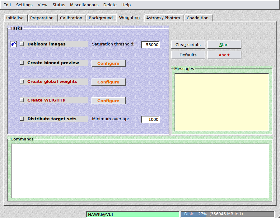
11. WEIGHTING

This section focuses on the determination of individual weight images that will be used in the final coaddition. In addition, you can perform a cosmetic correction of blooming spikes, and obtain some binned preview images for quick visual inspection of your data set. Satellite trails and other bad areas can be masked manually.

11.1. Debloom images

This is a purely cosmetic task and should only be used if you plan to publish a pretty picture based on your data. You should not base a scientific analysis on images that underwent this task. It will replace all pixels with values above the saturation threshold with values estimated from the local neighbourhood, i.e. remove blooming spikes. The profiles of saturated stars are significantly corrupted afterwards.

Filename extension: Images will have the character D appended to their filenames, e.g.

NGC1234_1OFCD.fits

11.1.1. Parameters

Saturation threshold: Pixels with values higher than this threshold will be interpolated.

11.2. Create binned preview

This task calculates binned images of the data. In case of multi-chip cameras all chips of one exposure are collected and arranged in the correct manner, such that you can see them all at once. Both FITS and TIFF versions are calculated, the latter can easily be eyeballed in your favourite image viewer programme. The binned versions are stored in BINNED_FITS and BINNED_TIFF sub-directories.

11.2.1. Parameters

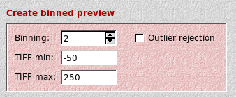
• Binning: The binning factor.
• Outlier rejection: Optionally, an outlier rejection can be switched on for the data binning. The 10% highest and 10% lowest pixels in the binning stack will then be rejected. If your data has a lot of hot pixels this will result in a much cleaner binned image.
• TIFFmin / TIFFmax: The TIFF version of the binned FITS image has a dynamic range of only 8 bit. You must therefore specify the black- and the white-point, i.e. pixels with values below TIFFmin are represented black, and those above TIFFmax are white. Since the sky background varies from exposure to exposure, this would lead to a very inhomogeneous representation. Therefore the mean value of the binned exposure is subtracted before conversion to TIFF (this does not happen for the binned FITS). TIFFmin should therefore be negative, and TIFFmax positive. This can require some trial and error in order to obtain a pleasing result. As a guide line, TIFFmax should be about 5-10 times larger than the absolute value of TIFFmin.

11.2.2. User-defined multi-chip cameras

Users of single-chip cameras can ignore this section.

The idea behind the binned images is to offer the user a visual representation of the data that displays all chips in a multi-chip camera at once. Like that chips affected by a satellite trail can be readily identified, or the quality of the pre-reduction verified (e.g. defringing, background subtraction, gain correction etc…).

This requires that THELI knows how to arrange the individual chips of a multi-chip cameras. If you defined a new instrument and you want to use this task, then you must manually create the following two files:

Chip configuration

The spatial distribution of the chips in your instrument (let’s assume it is called SOMEINSTRUMENT) must be stored in

~/.theli/scripts/album_SOMEINSTRUMENT.conf

This file must start with a commented header line, followed by one line for each chip defining the x and y position of its lower left edge at full resolution. In other words, think of your detector mosaic arranged in a global pixel grid. Then you would write down the x and y coordinates of the chips’ lower left edges, starting with chip 1 and ending with chip n. For WFI@MPGESO, an camera with 8 CCDs,

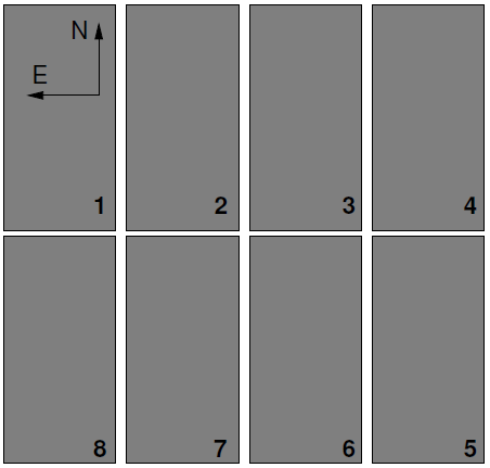
album_SOMEINSTRUMENT.conf looks like

#
1    4150
2100 4150
4200 4150
6300 4150
6300 1
4200 1
2100 1
1    1

Binning script

The configuration file created above must be loaded by an instrument-specific binning script. You can use any of the pre-defined make_album_xxx.sh scripts located in

THELI/gui-<version>/scripts/

as a template. Copy and rename it to

~/.theli/scripts/make_album_SOMEINSTRUMENT.sh

There is only one part in the script that needs to updated, the call to a function ${P_ALBUM}. It needs the total unbinned size of the mosaic in pixels (no precise value are needed, just round it up to the next 100 or so), and each chip as an individual argument. In case of WFI@MPGESO the corresponding part of the script reads

${P_ALBUM} -f ${DIR}/album_${INSTRUMENT}.conf ${ARGUMENT} -b ${V_WEIGHTBINSIZE} \
-p -32 8500 8300 \
${BASE}1$3.fits \
${BASE}2$3.fits \
${BASE}3$3.fits \
${BASE}4$3.fits \
${BASE}5$3.fits \
${BASE}6$3.fits \
${BASE}7$3.fits \
${BASE}8$3.fits \
> BINNED_FITS/${BASE}$3mosaic.fits

Herein, “8500 8300” would be the mosaic size in pixels (the -p -32 must not be changed), and then follow eight lines for each of the eight chips. If your camera has only four chips, you’d simply remove the lines for chips 5-8. If your camera has more, just add more.

Note

The order of chips in make_album_SOMEINSTRUMENT.sh must be the same as in album_SOMEINSTRUMENT.conf.

11.3. Create global weights

Each image that enters the coaddition process has its own, individual, weight map. The basis of the latter is the normalised flat field telling how much information a particular pixel contains compared to all other pixels. Therefore pixel weights are not simply 1 for good pixels and 0 for bad pixels, but have a floating point representation.

Optionally, static pixel defects and other features that should be masked can be set to zero, forming the global weight that is the same for all images of a particular detector. This global weight is individually modified in the Create WEIGHTS task below.

The globalweight is stored as

/mainpath/WEIGHTS/globalweights_1.fits

11.3.1. Parameters:

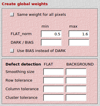
• Same weight for all pixels: If you don’t have a master flat for the basis of the global weight, or don’t want this approach for other reasons, you can force all pixels in the global weight to have a value of “1.0”. Bad pixel detection as described above based on a master dark can still take place.
• Flat norm: Pixels with values outside the [min:max] interval in the normalised flat field are set to zero in the global weight. In this manner significantly vignetted regions and other underexposed detector areas can be masked. If left empty, default values (min=0.6, max=1.5) will be used.
• BIAS/DARK: Optionally, the master dark can be used to identify bad pixels. Pixels with values outside the [min:max] interval will be set to zero.
• Use BIAS instead of DARK: If you don’t have a master dark, the master bias can be used to identify bad pixels. However, this works less reliably then with a master dark.

Defect detection

Warning

Defect detection will NOT work with CMOS detectors, such as near-IR HAWAII arrays or DSLR cameras, NOR will it work with amateur astronomer cameras using a Bayer color filter matrix.

THELI can attempt to identify bad rows, columns, and clusters of bad pixels running the flatfield through a highly sensitive feature detection filter. The flatfield is divided by a smoothed version of itself, yielding a normalised detection map with all illumination patterns removed. For the detection of bad rows (columns) a mean row (column) is calculated in an iterative manner with internal outlier rejection, and individual rows (columns) are compared against it.

• Smoothing size: This is the size of the smoothing kernel. It should be chosen comparatively small, such as a few 10 pixels.
• Cluster tolerance: Pixels in the detection map are masked if they deviate by more than this fraction from their local neighbourhood.
• Row tolerance: If a row deviates by more than this fraction from the mean row, it will be masked. Useful thresholds are around 0.01-0.02.
• Row tolerance: If a column deviates by more than this fraction from the mean column, it will be masked. Useful thresholds are around 0.01-0.02.

11.4. Create WEIGHTS

In this step the global weight map is modified for each image individually and stored in the WEIGHTS directory.

11.4.1. Parameters

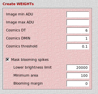
• Image min (max) ADU: Pixels in the image with values below (above) this threshold will be set to zero. In this way you can explicitly mask pixels that are e.g. close to saturation, nonlinear, or suffer from other problems.

• Cosmics threshold: If you set this parameter (default for well-sampled images: 0.1) THELI runs a neural network algorithm over the image that has been trained to detect cosmics. The latter appear significantly sharper than the PSF in well-sampled images and can thus be masked (without running a computationally expensive comparison between all images). This approach breaks down for undersampled data, in which case the cores of stars will be masked. If you observe this in your stacked image (or in the individual weight images) then switch off this feature (i.e. leave the field empty). You can use an outlier detection algorithm during the coaddition instead to get rid off spurious pixels.
• Cosmics DT: The minimum S/N per pixel for a cosmic. The higher, the less cosmics will be detected. The default setting of 6 should be fine for most cases.
• Cosmics DMIN: The minimum number of connected pixels with S/N above Cosmics DT that make up a cosmic. The default setting of 1 should be fine for most cases. If DMIN is larger than 1, then individual hot pixels will not be masked anymore.

Mask blooming spikes: If you want to explicitly set the weight of pixels affected by blooming spikes to zero, activate this switch. The algorithm uses some adaptive statistics in order to deal with detectors where the saturation limit is spatially varying. The idea is that in a histogram of pixel values the brighter pixels are less and less common. However, once saturation kicks in, pixels bleed over into neighbouring pixels at specific ADU levels, which is recognisable as a pile-up in the histogram at high values. This algorithm attempts to detect this turn-up by means of comparison with the number of pixels with lower ADU values. This turn-up can be different from chip to chip, and even vary within a CCD.

• Lower brightness limit: This is NOT the threshold above which pixels are considered to be part of a blooming spike. This value should be chosen such that it is well above the background level (in order to remove the latter from the pixel statistics), but still significantly lower than the lowest value of pixels being part of a blooming spike (see the description above). You could set it about twice as high as the typical background level, or about to 30-40% of the saturation level.
• Minimum area: This is the number of pixels a blooming spike should at least consist of in order to be masked.
• Blooming margin: If the values of pixels in blooming spikes vary depending on detector position, then you should set this parameter to a value other than zero. For example, if you observe variations of 5000 ADU between the top and the bottom of the CCD, you should set this parameter to 5000. The dynamic range within which pixels are masked is therefore increased.

11.4.2. Masking satellites

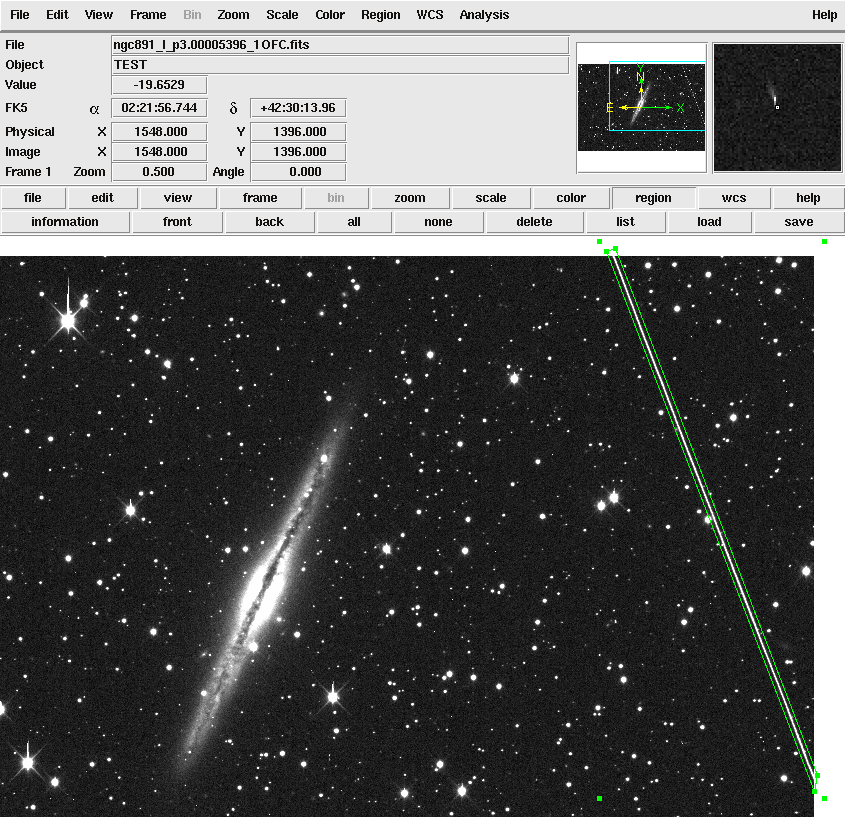
Satellites can be masked using ds9 polygons:

1. Open the image containing a satellite track in ds9

2. From the main menu, select Region -> Shape -> Polygon

3. Click in the image and drag a rectangle with the mouse button pressed. When finished, click into the rectangle.

4. Point the cursor precisely over one of the vertices, then click on it and pull it towards the satellite trail. Repeat with the other vertices until the trail is fully enclosed in the polygon. If you need more vertices, just click onto a connecting line.

5. Click on Region -> Save to save the polygon mask. Save it in the same directory as your images, with the same name as the image but without the status string. For example, if the image file name is

   NGC1234_3OFC.fits
   

   then the ds9 mask should be called

   NGC1234_3.reg
   

   When saving the mask, ds9 will ask you in which format to store it. Choose REG, then ds9 and physical.

The masks created in this manner will be taken into account when the individual weight map are created. They will be slightly reformatted and moved to

SCIENCE/reg/*.reg

You can mask any image artifact in this way using arbitrarily shaped ds9 polygons.

11.5. Distribute target sets

If you observed different targets in the same filter in a given night, you will probably have kept them in the same directory up until now (at least if you observed in the optical). The following steps however (astrometry etc.) must be performed on each pointing individually, and thus different targets must be moved to separate SCIENCE directories.

If images overlap by more than minimum overlap pixels (linear extent), then they are considered to belong to the same pointing. Otherwise they will be moved to newly created set_i directories (in the directory tree at the same level as the SCIENCE directory in which they lived before this task run). The set_1 directory will be automatically inserted in the Initialise section.

The largest value accepted by minimum overlap is 1024.