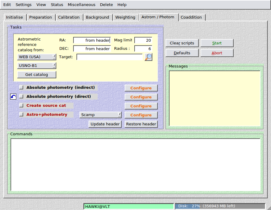
12. ASTROMETRY / PHOTOMETRY
In this section astrometric and photometric solutions are obtained, i.e. images are registered to sky coordinates and are (optionally) flux calibrated. Note that the determination of an absolute photometric zeropoint is optional. The relative zeropoint of exposures, i.e. transparency variations etc are always determined. Results are written to separate FITS headers which are later-on read during the coaddition process.
12.1. Astrometric reference catalog
12.1.1. Making the right choice
This little section controls the download of the astrometric reference catalogue. While programmes such as scamp can do that internally and thus invisible to the user, there are numerous cases where such an approach is problematic. The principle behind all astrometric solvers is to match a catalog of reference sources to catalogs containing sources in your images. In order to identify the correct solution, a certain minimum contrast (in the one or other statistical sense, depending on the method) is required. This can fail in several situations:
- You observed a field at low galactic latitude (i.e. in the milky way) with an extremely high source density. If you download too to many (i.e. too faint) sources, then the solution space is so densely populated that the right solution is difficult to recognise (and the computational overhead is very large).
- You observed a field at high galactic latitude with very low object density. Then you want your astrometric reference catalog to be as deep as possible in order to have sufficient overlap with your image catalogue.
- You observed with a very large telescope and most stars in your reference catalogue are saturated in your images. Or the field of view is so small that none or only very view reference sources overlap with it. In this case you have to consider a deeper reference catalog, or you create one using secondary imaging of the area with a smaller telescope yielding deeper catalogs than what is available in online databases.
- Wavelength mismatch: You observe a region with high galactic extinction (e.g. a dark cloud) in the optical, and the reference catalog does not contain any sources for that area. You might consider switching to a near-IR catalog.
- Wavelength mismatch: You want to match a very blue optical catalog to a near-infrared reference catalog. They hardly have any targets in common and thus the astrometry fails.
- One of the online servers is down and you have to switch to a different one.
- Any combination of the above, or something else.
Astrometry in THELI usually works fine with the default settings, provided that the information in your FITS headers is halfway reliable. You can try and run it blindly, and if it fails then fine-tune some settings.
The enumeration above shows that in the end the success of the astrometric solution depends on the overlap between the reference catalog and the image catalogs. That is, you should not only think of the reference catalogue but also of the source catalog creation as the latter allows you to control how many sources are detected in your images.
You should aim for 100-1000 sources per chip, in the reference catalog as well as in the image catalogs. THELI will also work with a few 10s or with 10000+ per chip, but if you push it to the limits it can become difficult.
12.1.2. Parameters

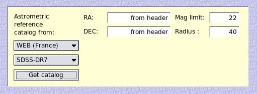
RA / DEC: This is only needed if your FITS header does not yet contain astrometric coordinates, or if these are significantly offset from the correct value. Otherwise the centre for the reference catalog will be determined from the FITS header.
Resolve target: Enter the name of your target. Once you click the button with the magnifying glass, THELI sends a query to the Simbad, NED and VizieR databases to retrieve the target’s coordinates (if not already contained in the FITS header).
Note
After entering coordinates, THELI will prompt you with a notification window when you hit the Start button. Therein, you have three options:
- Update RA/DEC: Will overwrite the CRVAL1/2 keywords.
- Update RA/DEC, reset CD matrix: Will overwrite the CRVAL1/2 keywords and reset the CD matrix (CDi_j keywords) to a North up and East left orientation.
- Leave header unchanged: Select this option if you changed your mind and do not want any changes being made to the FITS header.
Mag limit: Only sources brighter than this limit will be retrieved. This is your control over the density of the reference catalog.
Radius (optional; in arcminutes): Determined automatically, taking into account detector size and dither offsets. Objects within this radius of the nominal coordinates in the FITS header (or those entered manually) will be downloaded.
- Source: Choose from 9 different download locations. If you have problems with one of them, switch to another. You can also choose IMAGE, in which case you will be presented with a file selection dialogue from which you can pick an astrometrically calibrated image that covers your field of view. In that case you have to provide the usual Sextractor detection thresholds DT and DMIN (defaulted to 10 each).
- Catalog: Choose from 8 different reference catalogs
Once your selection is made, click on Get catalog to retrieve the reference catalog. The number of sources found will be displayed.
12.1.3. Available reference catalogs
Choose from one of these astrometric reference catalogs:
| Catalog | Mag-limit | Remarks |
|---|---|---|
| SDSS-DR9 | 23.0 | Covers 14000 sq.deg around the northern galactic cap |
| ISGL | 21.0 | Initial Gaia Source List, allsky, heterogeneous but clean |
| PPMXL | 21.0 | Combines USNO-B1 with improved astrometry and 2MASS |
| USNO-B1 | 21.0 | 0.3”-0.4” rms uncertainty; can exhibit large systematics |
| 2MASS | 18.0 | Near-infrared, low systematics |
| URAT1 | 18.5 | UCAC4 successor down to about DEC=-10 |
| SPM4 | 17.5 | Yale/San Juan astrometry catalog, deeper than UCAC4 |
| UCAC4 | 16.5 | Good proper motions, all CCD based |
| GSC-2.3 | 19.0 | |
| TYC | 11.0 | The TYCHO catalog |
| ALLSKY | 10.0 | Based on GSC-2.3, filtered to mag<=10. Comes with THELI as downloading huge areas from CDS often resulted in incomplete sky coverage. |
TYC and ALLSKY should only be used for calibration of extremely wide fields (obtained e.g. with photo lenses) with very large pixel scale (much larger than 1.0”/pixel).
12.2. Absolute photometry
There are two ways to perform absolute photometry: an indirect approach using external standard star fields, and a direct approach using sources with known brightness in the field of view. THELI supports both methods, returning the photometric zeropoint ZP (for an image normalised to an exposure time of 1s).
12.2.1. Before you start
Doing absolute photometry in THELI is simple. However, note that the flux calibration must be obtained BEFORE object catalogs are created and BEFORE they run through astrometry and relative photometry. Otherwise the zeropoints cannot be propagated properly.
Indirect approach: The standard star field has to be calibrated astrometrically to identify the reference stars unambiguously. This requires the download of a reference catalog (happens automatically), the creation of object catalogs, and a (simple) astrometric solution (no distortion fitting).
In some cases, such as the near-IR, only very few sources will be visible in the field, perhaps just the reference star itself. An astrometric solution cannot be obtained in the usual way. If the initial WCS astrometry in the FITS header is accurate enough, the objects can still be matched with the photometric reference catalog (see below).
Direct approach: Astrometric and photometric reference catalogs must be downloaded for the target area, followed by catalog creation and an astrometric solution (such that targets in the field can be identified with those in the reference catalogs).
Note
Obtaining the ZP requires catalog creation and astrometric solutions. The configuration parameters for these tasks will be taken from the configurations of the Create source cat task and from the Astro+photometry task described further below. You must make sure that these settings are sensible, otherwise the absolute photometry will fail. It is a good idea to familiarise yourself with these two tasks first before you dive into absolute photometry.
12.2.2. Indirect approach: using external standard stars
Prerequisites
You must have observed at least one field with photometric standard stars in the same filter as your observations. Select the following standard star catalogs for observations in these filters (note that the filter curves of these standard stars may not be the same as the ones used in your filter set. Check the pertinent publications for more details).
FILTER Catalog UBVRI Landolt (Landolt 1992) UBVRI Stetson (Stetson 2000) ugriz Stripe82 (Smith 2007) u’g’r’i’z Stripe82 (Smith 2007) JHK MKO (Leggett 2006) JHK HUNT (Hunt 1998, aka ARNICA) JHKKs PERSSON (Persson 1998) JHKKs PERSSON_RED (Persson 1998) YJHKLM JAC (WFCAM+MKO+MKO_LM) LM MKO_LM (Leggett 2003) Your observations must have been conducted in one of the filters listed in the table above
The night should have have been photometrically stable, i.e. no change in transparency at a given airmass.
The standard star field(s) should have been visited several times at night at significantly different airmasses for extinction calculation. You should go down from about 1.0 all the way to 1.8 or 2.0, covering several steps in between.
You may include standard star and target observations from many different nights. An independent solution will be calculated for each night.
Before you start reducing your target data, create a separate directory at the same level in the directory tree as the SCIENCE directory containing your main target. Include the name of your standard star directory in the Initialise section in the STANDARD field. When you reduce your target observations, the standard data will be processed too, including the same calibration files (master bias, master flat, if applicable also background correction) as the target observations.
Note
You can collect different standard star fields (taken in the same filter) in the same STANDARD directory. THELI will automatically obtain a photometric solution for each night.
Note that if your data set extends over several nights, it is sufficient for an absolute photometric calibration if only one night was calibrated successfully.
Parameters
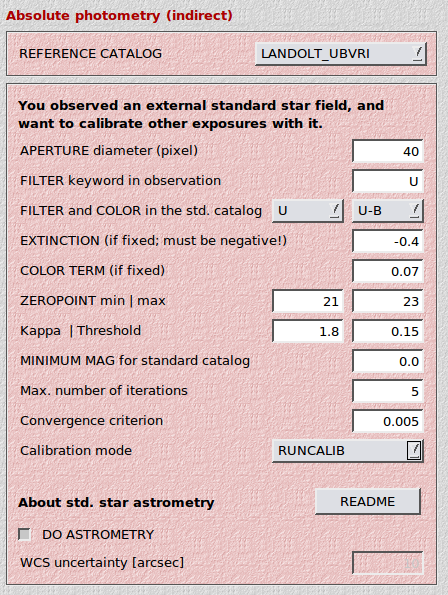
- REFERENCE CATALOG: Choose one that matches your filters
- FILTER keyword in observation: The name of the filter in which you observed.
- FILTER name in the standard catalog: The name of the filter in the standard star catalog which matches your filter
- COLOR INDEX in the standard catalog: The color term for the photometric solution is based on the colors in the reference catalog, i.e. you do not have to observe the standard star field in different filters. Select the color index that matches your observations, respectively the corresponding filter in the standard catalogue.
- EXTINCTION: If your standard star observations do not cover a sufficiently large range in airmass, then the atmospheric extinction cannot be estimated reliably from the data. In this case the value entered here will be taken as the extinction. It must be negative. If no value is entered, the default of -0.1 will be used.
- COLOR TERM: If the color term cannot be determined reliably from the data, then the value entered here will be used. If left empty, it is set to 0.0.
- ZEROPOINT min | max: THELI will initially reject zeropoints that lie outside this interval (to avoid catastrophic outliers)
- kappa | threshold: The kappa-sigma cut-off for the outlier rejection (in units of sigma). Furthermore, objects with a ZP lower than threshold (in mag) below the fit will be rejected as well during iteration. Sources may re-enter the fit in the next iteration.
- MINIMUM MAG for standard catalog: Stars brighter than this magnitude will not be used for the fit.
- Max. number of iterations: How many iterations are done for the fit. Anything from 0 to 10 may be sensible, depending on the quality of your data.
- Convergence criterion: Convergence is assumed if all three of ZP, the extinction coefficient and the color term change by less than this (absolute) amount between iterations. usually, 0.005 to 0.01 make sense.
- Calibration mode: RUNCALIB calculates one common photometric solution for all standard star observations taken over several nights. NIGHTCALIB calculates nightly photometric solutions.
- Do astrometry for standard star fields: This is switched on by default. If the source density is too low to obtain an astrometric solution, you may switch this setting OFF, and provide an estimate of the astrometric uncertainty in arcseconds. THELI will then attempt to match the object catalogs with the photometric reference catalogs, assuming the initial WCS solution in the FITS headers is not too far off.
Four different photometric solutions are calculated:
- 3-parameter fit: extinction, color-term and ZP are estimated
- 2-parameter fit: extinction and ZP are estimated, color term is fixed
- 2-parameter fit: color term and ZP are estimated, extinction is fixed
- 1-parameter fit: ZP is estimated, extinction and color term are fixed
The results are stored in a calib/ sub-directory, in form of a table and a graphical display. Based on these you may fine-tune your manual selection of a fixed extinction and color term coefficient, and then re-run the task. The zeropoints and coefficients will be written into FITS headers. If no ZP is found, the keyword is set to -1.
The following display of the four solutions is created and stored in the calib/ sub-directory. The left column shows the ZP as a function of airmass, AFTER correcting for the color-term determined by the same fit. The right column shows the ZP as a function of object color, AFTER correction for extinction. Red crosses indicate data points that were rejected for the final fit. Note that depending on the best-fit found, different data points may be rejected, and that the distribution of points and the y-axis range may change between fit types (as we apply color and extinction correction from the fit). Remember which fit suits you best. You will be asked during the final astrometry of your science fields which solution to take.

Note that if your data set extends over several nights, it is sufficient for an absolute photometric calibration if only one night was calibrated successfully.
12.2.3. Direct approach: using field sources with known brightness
The other possibility for absolute photometric calibration is to determine the zeropoint (ZP) directly from the data. You do not need observations of an external standard star field.
Warning
Direct photometric calibration in THELI does not take into account color terms arising from different total throughput curves between your telescope/filter/camera combination and the one used for SDSS or 2MASS. If you need absolute zeropoints better than about 0.1 mag then you should consider fine-tuning the ZPs obtained with this method using a comparison of instrumental stellar tracks against those in the Pickels library.
Prerequisites
- Your field is covered either by SDSS (optical data) or 2MASS (for near-IR observations). SDSS has no all-sky coverage but a high density, whereas 2MASS covers the entire sky but is rather shallow.
- Your observations must have been conducted in one of the ugriz filters (SDSS), or in JHKs (2MASS).
Parameters

- REFERENCE CATALOG: Select either SDSS or 2MASS
- FILTER IN WHICH YOU OBSERVED: Select one of ugriz or JHKs
- MAX PHOTOMETRIC ERROR (mag): The maximum photometric measurement error of sources in your data that go into the fit.
- FITTING METHOD: You can select between ZP for each chip or ZP for entire mosaic. The latter assumes that the pre-processing went fine, in which case no zeropoint variations are expected across the field of view. If you choose to calculate a ZP for each chip, then all chips will be rescaled to the highest ZP found, and this ZP will be written into the FITS headers (i.e. the ZPs in the headers of different chips are identical).
Filename extension: After doing direct photometric calibration with FITTING METHOD = ZP for each chip, images have the character P appended to their filename extension, e.g.
NGC1234_1OFCP.fits
In all other cases no chip-specific treatment is necessary and thus no indication has to be made in the file names.
12.3. Create source cat
In order to detect objects in the images for astrometry and photometry purposes, THELI uses SExtractor. We encourage you to make yourself more familiar with this tool (see also the other links on the SExtractor website).
The task creates the following sub-directories:
- SCIENCE/cat : contains the binary object catalogs
- SCIENCE/cat/skycat : object catalogs for overlay in skycat
- SCIENCE/cat/ds9cat : object catalogs for overlay in ds9
- SCIENCE/cat/lownum : dodgy catalogs with too few sources end up here
12.3.1. Parameters
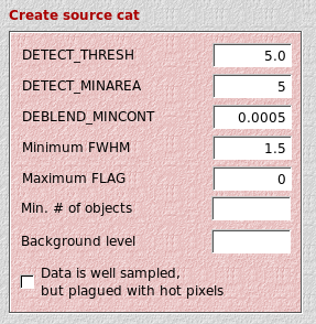
- DETECT_THRESH: The minimum S/N of a pixel above the background rms. If this value is decreased, fainter objects will be included in the catalogs. The lowest sensible value is about “1”, combined with DETECT_MINAREA=5. The default value is “5”. If your field is very crowded, consider rising it to 10 or higher.
- DETECT_MINAREA: The number of connected pixels with a S/N larger than DETECT_THRESH required for an object. The smaller this parameter, the fainter the objects included.
- DEBLEND_MINCONT: This is SExtractor’s internal deblending contrast. You can leave it at its default setting of 0.0005, unless you need to detect objects against a very crowded or structured background, such as a large spiral galaxy. You can e.g. make it as small as 0.00001. If a large number of detections e.g. in a globular cluster seems to shadow the right astrometric solution, increase it to e.g. 0.01, in which case less sources will be detected in the cluster.
- Minimum FWHM: Objects with a FWHM smaller than this value will be rejected from the catalogs. Normally you do not have to touch this setting and can leave it to its default setting of 1.5. THELI runs several filters over the object catalogs in order to remove spurious detections such as hot pixels. If your data is significantly undersampled, i.e. the FWHM is less than two pixels broad, then you should decrease this parameter to a sensible lower limit. Values less than about 0.7 or 0.8 do not make much sense.
- Saturation level: At this level saturation occurs. If nothing is entered, then THELI will assume a conservative value of 50000 ADU. For 12bit cameras such as DSLRs this value should be set much lower. For near-IR detectors it can also be much lower after background subtraction, but also much higher if on-chip coadding took place.
Maximum FLAG: Per default, THELI keeps only objects that were not flagged (FLAG=0) as problematic by SExtractor. However, there are cases when you need to include flagged objects as well in order to arrive at an astrometric solution. For example, for mildly saturated stars one can still determine a good centroid, which can be very helpful if the faint end of the astrometric reference catalog is close to saturation in your images. Similar considerations apply to objects close to image borders, etc.
Quoting from the SExtractor manual: The FLAGS parameter contains all the extraction flags as a sum of powers of 2:
- FLAGS=1: The object has neighbours, bright and close enough to significantly bias the MAG_AUTO photometry, or bad pixels (more than 10% of the integrated area affected)
- FLAGS=2: The object was originally blended with another one
- FLAGS=4: At least one pixel of the object is saturated (or very close to)
- FLAGS=8: The object is truncated (too close to an image boundary)
- FLAGS=16: Object’s aperture data are incomplete or corrupted
- FLAGS=32: Object’s isophotal data are incomplete or corrupted
- FLAGS=64: A memory overflow occurred during deblending
- FLAGS=128: A memory overflow occurred during extraction
For example, an object close to an image border may have FLAGS=16, and perhaps FLAGS=8+16+32=56.
Min. # of objects: If a catalog contains less objects than this number, then the catalog and the corresponding image are moved to lownum sub-directories and will not enter astrometry and coaddition.
Background level: SExtractor usually gets the background level correctly. However, it may fail if a large number of NAN pixels is present, and then the object detection will also fail. In this case you can manually set the background level, assuming it is the same for all images (I was forced to use this setting only once, for background-subtracted Pan-STARRS images).
Data is well sampled, but plagued with hot pixels: Activate this switch if your images have REALLY A LOT OF hot pixels and/or other strange small-scale features that might be mistaken for real objects. A lot of means comparable to or more than real objects. This probably makes only sense for HAWAII near-infrared arrays with very bad cosmetics. Optical astronomers can ignore this switch.
12.4. Astro+photometry
5 different methods are available for astrometry. The first two methods, Scamp and Astrometry.net, perform automatic mosaicing, whereas the two shift approaches do not base their solution on WCS coordinates. All but the last method (Header) perform relative photometry as well, i.e. measure transparency variations in a series of images.
Scamp: The preferred method, fast, creates meaningful check-plots. Can be difficult to find a match with the reference catalog if both the position as well as the position angle (and possibly a flip) are highly uncertain or unknown.
Astrometry.net: Matching is done differently as compared to Scamp. Relative zeropoints, and optionally distortion, is calculated afterwards with Scamp (automatically, using the preset Scamp parameters). Checkplots are provided by Scamp. Comparably fast as Scamp.
Shift (float/int): A very simple solver that calculates image shifts only. No rotations and no WCS parameters are involved. The shifts are computed in pixels with respect to the first image in the series. This is only useful for mid-IR data where only very few or only one object at all is visible. The astrometry of the coadded image will NOT be accurate as no comparison with reference catalogs is made. If you use the integer approach, only integer pixel shifts and no resampling will be performed during coaddition. This method cannot be used for mosaicing.
Header: This will simply copy the unchanged raw zero-order solution (CRVAL, CRPIX, CDi_j) present in the FITS headers, albeit without distortion terms. This can be chosen if the raw data already has a good astrometric solution in the headers (e.g. determined by other software) and you prefer to use this over the THELI solution.
Warning
No relative photometric calibration will be done when chosing this method.
All methods create separate FITS header files with the relevant astrometric (and, if applicable, photometric) information. The headers are stored in
SCIENCE/headers/
Update header: Writes the zero-order astrometric solution (CRPIX, CRVAL, CD-matrix) into the FITS headers. This is usually not necessary unless you need accurate sky coordinates for some reason. The only such reason in THELI is when you have to extract a background estimate from a small sky section and you want this area to be exactly the same despite a dither pattern. See the sky subtraction for details.
Restore header: Restores the previous FITS headers if a zero-order solution was written into them using Update header.
12.4.1. Scamp
We strongly recommend to have a look at the scamp manual for details as of how Scamp works.
The following parameters are available.

- POSANGLE_MAXERR: Maximum uncertainty in the position angle (up to 180 degrees)
- POSITION_MAXERR: Maximum uncertainty in the pointing in arcminutes
- PIXSCALE_MAXERR: Relative uncertainty of the pixel scale
DISTORT_DEGREES: Distortion polynomial order. Distortion in the sense of Scamp is a variation of the pixel scale as a function of position. All other (linear) transformations are explicitly modelled as such and encoded in the CD matrix. The distortion degree entered in this field means:
- distort=1: no distortion modelled; pixels have the same scale everywhere
- distort=2: pixel scale may vary linearly across the chip (makes sense only for multi-chip cameras)
- distort=3: pixel scale may vary quadratically
- distort=4: cubic terms are included …
Scamp can also make use of higher distortion polynomials, but they get increasingly more unstable and require a large number of sources.
FGROUP_RADIUS: The maximum angular separation between to pointings. If two images are further apart, then independent astrometric solutions will be calculated for them.
CROSSID_RADIUS: The search radius (in arcsec) for cross-identifications. This value can remain at its default setting of 2, unless the pixel becomes larger than 0.7 arcsec/pixel. In the latter case, THELI sets

ASTREF_WEIGHT: In Scamp the object catalogs and the reference catalogs have equal weights in the solution process. Some cases may require to put more weight on the reference catalog. If your reference catalog is very precise and accurate to within e.g. 1/5th of a pixel of your camera, then you may choose a very large weight such as 10 which would make the reference catalog control your solution. Usually, the resolution of the camera is equal to or better than the uncertainty of the reference catalog. The default value for this parameter is 1.
SN_THRESHOLDS (low|high): Minimum S/N of a source to be kept in Scamp (low), and the minimum S/N for some high-S/N statistic calculations (high).
Additional DISTORT_GROUPS | DEGREES | DISTORT_KEYS: In almost all cases one can ignore these three settings (i.e. leave them empty). One would enter here a comma-separated list of additional distortion groups, degrees and keywords. DISTORT_KEYS would also accept FITS keywords, which must be preceded with a “:”.
Example: A set of images with arbitrarily distributed position angles is being stacked, and it turns out the distortion pattern is a linear function of the position angle. One would then define a new distortion group, DISTORT_GROUPS=2, with DISTORT_DEGREES=2 and DISTORT_KEYS= :POSANGLE” to reflect the dependence of the distortion of the position angle. For more details see the *Scamp manual.
ASTRINSTRU_KEY: The FITS header keyword used to identify exposures for which one astrometric solution should be calculated. The default value is FILTER, meaning that images with the same FILTER header keyword will have one solution calculated. Images with different values in those keywords will get their own solution. You can add several comma-separated keywords in order to break down the astrometric solution into smaller groups. If you want to calculate one solution for images taken in different filters, then just enter a string that does not exist as a keyword in the FITS header, such as “none”.
- PHOTINSTRU_KEY: The FITS header keyword used to identify exposures for which one photometric solution should be calculated. The default value is FILTER, meaning that images with the same FILTER keyword will have one solution calculated. If you want to calculate one solution for images taken in different filters (for flux-normalisation purposes for example, e.g. difference imaging), then just enter a string that does not exist as a keyword in the FITS header, such as “none”.
- STABILITY_TYPE: INSTRUMENT can be used if one is sure that the distortion pattern does not change during a series of exposures. EXPOSURE should be used if all parameters shall be determined individually per exposure (and chip).
- MOSAIC_TYPE: Quoting from the Scamp user manual: Scamp can
manipulate mosaics in a number of ways to perform the matching of sources
on the sky, and the astrometric calibration itself. For single-chip cameras
only the UNCHANGED mode makes sense.
- UNCHANGED: The relative positioning of detectors on the focal plane, as recorded in the WCS keywords of the FITS headers, is assumed to be correct and constant from exposure to exposure. Matching with the reference catalogue will be done for all the detectors at once.
- SHARE_PROJAXIS: The relative positioning of detectors is assumed to be constant and correct, but the different extensions within the same catalogue file do not share the same projection axis (the CRVAL FITS WCS keywords are different): although this does not prevent Scamp to derive an accurate solution, this is generally not an efficient astrometric description of the focal plane. This option brings all extensions to the same centred projection axis while compensating with other WCS parameters.
- SAME_CRVAL: Like SHARE_PROJAXIS above, brings all extensions to the same centred projection axis (CRVAL parameters), but does not compensate by changing other WCS parameters. This option is useful when the CRPIX and CD WCS parameters are overridden by some focal plane model stored in a global .ahead file.
- FIX_FOCALPLANE: Applies first a SHARE_PROJAXIS correction to the headers and then attempts to derive a common, median relative positioning of detectors within the focal plane. This mode is useful to fix the positions of detectors when these have been derived independently at each exposure in an earlier not-so-robust calibration. A minimum of 5 exposures per astrometric instrument is recommended.
- LOOSE: Makes all detector positions to be considered as independent between exposures. Contrary to other modes, matching with the reference catalogue will be conducted separately for each extension. The LOOSE mode is generally used for totally uncalibrated mosaics in a first Scamp pass before doing a FIX_FOCALPLANE.
- Which focal plane: What Scamp should assume about the detector mosaic:
- Use default FP: Use the focal plane model implemented in THELI
- Create new FP: Create a new FP model based on your data (will not replace the default model)
- Do not use FP info: Do not assume anything about the focal plane
- Match flipped images: If set, then Scamp will attempt to match flipped images, i.e. the image is flipped with respect to what its CD matrix says.
- Match WCS: If set, then Scamp will attempt to match the image catalogs with the downloaded source catalogs. This can be deactivated if the astrometric accuracy in the FITS header is better than CROSSID_RADIUS (see above), and no ambiguities exist at that level between source and reference catalog.
12.4.2. Astrometry.net
For more information about this tool visit www.astrometry.net.
The following parameters are available.
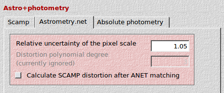
- PIXSCALE_MAXERR: Relative uncertainty of the pixel scale
- Distortion polynomial degree: Currently deactivated, as SWarp does not understand SIP polynomials
- Calculate SCAMP distortion after ANET matching: The distortion output of ANET is not understood by SWarp (image coaddition). To still get distortion correction, you can run Scamp after ANET has done the matching. In this case the matching function of Scamp is deactivated. In addition, Scamp will also calculate the relative photometric zeropoints as usual, which are not provided by ANET. Hence this checkbox should always be activated. THELI will use the distortion polynomial degree (and all other Scamp parameters) as entered in the corresponding configuration dialog.
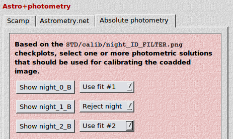
12.4.3. Absolute photometry
Here you will find a list of up to 7 nights during which standard stars were observed and a photometric solution obtained (if any). You may reject a night, or select one of the four different fit types.
12.5. Trouble-shooting Scamp
It happens that Scamp returns a wrong astrometric solution without recognising it. This usually happens when the images were not correctly matched to the sky. You do not need to go through a possibly lengthy coaddition to find out if the solution was good or not. In most cases it is sufficient to have a look at the various check-plots created by Scamp. You can find them in
SCIENCE/plots/
In the same directory is also a scamp.xml file with further valuable information that can help you identify trouble-making images and other issues. In order to look at the XML file with firefox, you must first enter in the address field
about:config
and then locate the following parameter and set it to false:
security.fileuri.strict_origin_policy = false
Otherwise the XML file will not be displayed correctly.
If you can’t get it done with Scamp, you may equally well try Astrometry.net which uses a different matching algorithm that is superior if WCS parameters such as pointing and position angle and a possible flip are unknown.
12.5.1. Interpreting Scamp check-plots
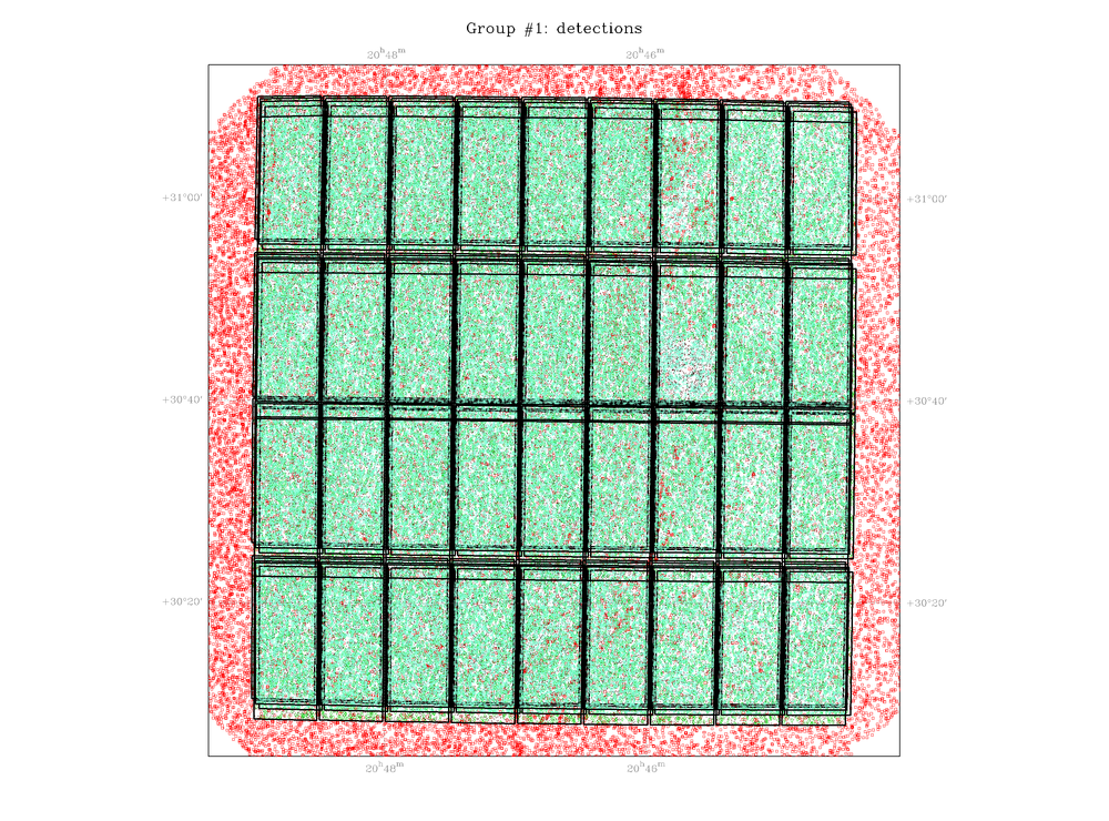
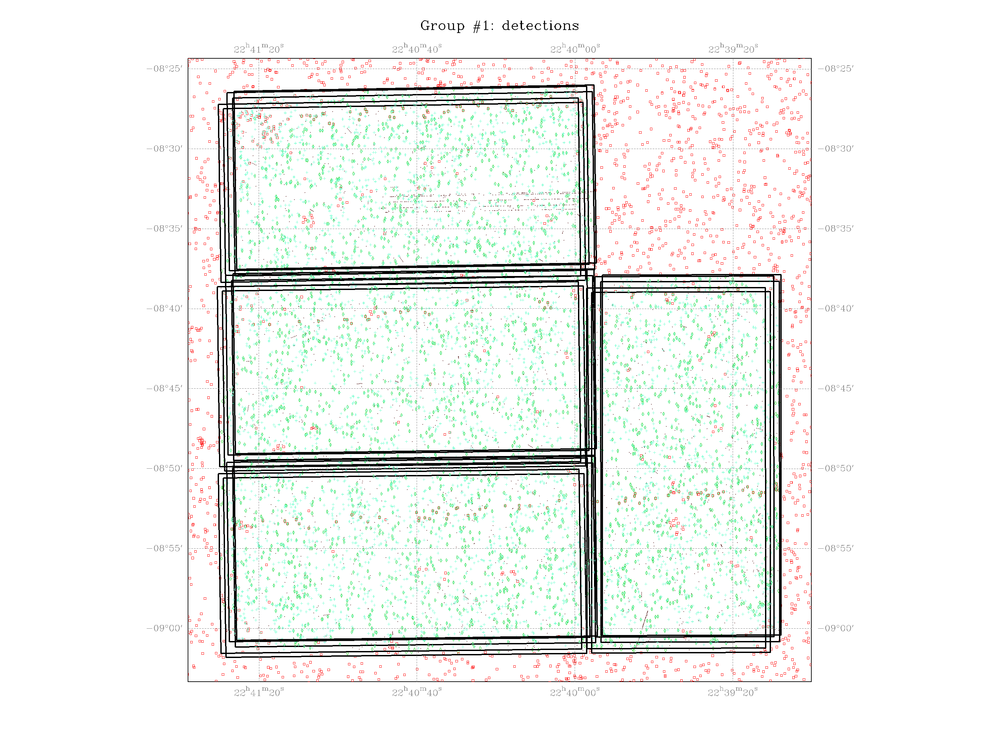
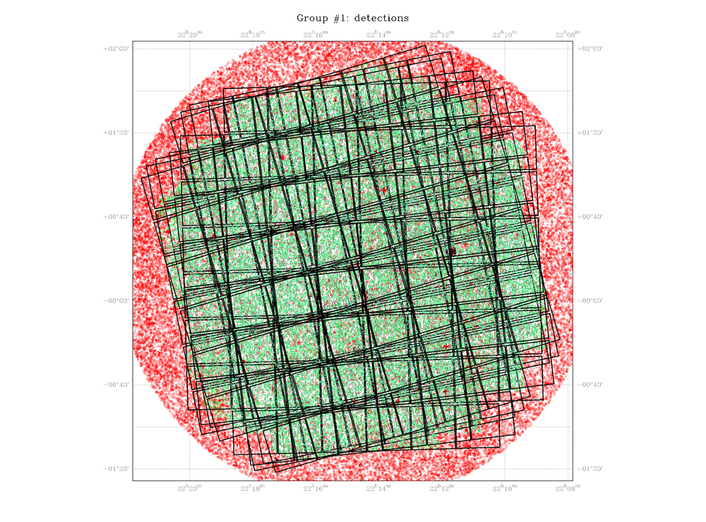
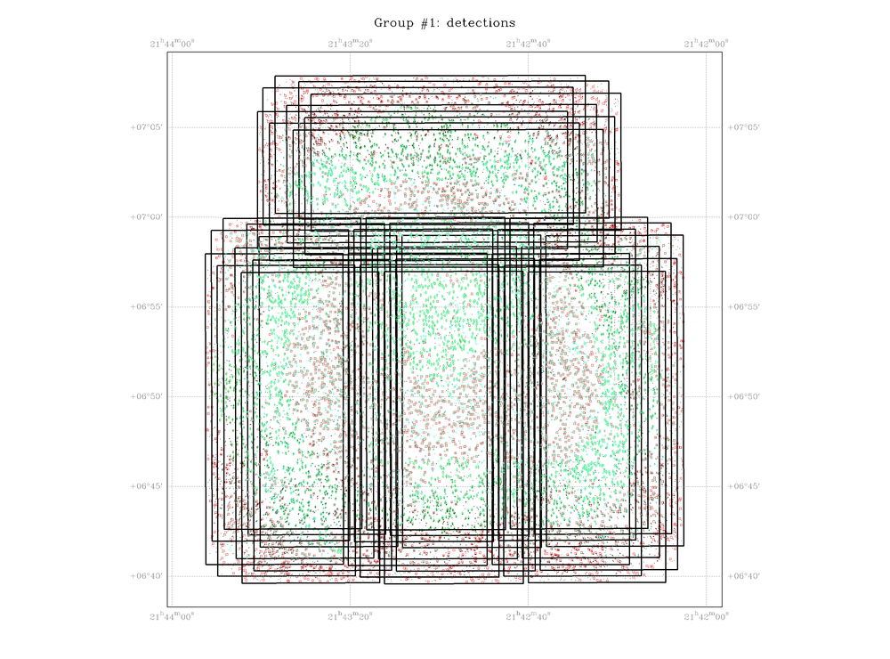
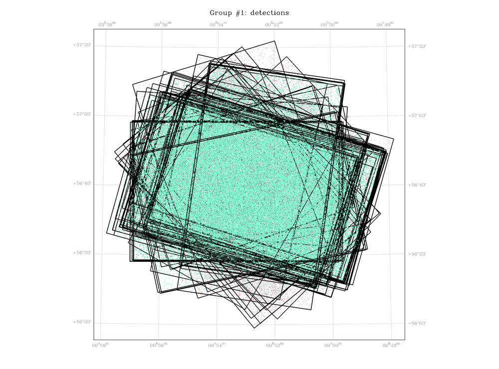
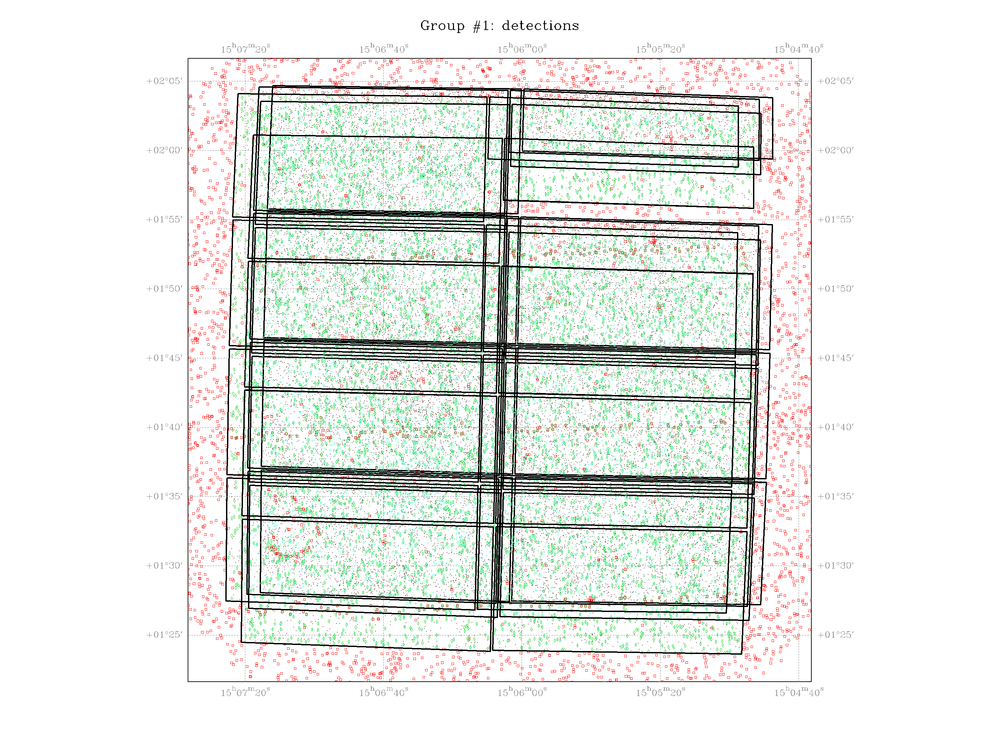
Image distribution on the sky: fgroups
This should be the first plot you should look at. It displays the dither pattern together with unmatched (red) and matched (green) reference sources. You should recognise your dither pattern here.
Good fgroups plots
- Example 1: Megacam@CFHT
- Example 2: A mosaic of ACS/HST images. The overlap with the ground-based reference catalog is not very compelling, but sufficient.
- Example 3: WFC@INT (wide-field camera at the 2.5m Isaac Newton Telescope)
- Example 4: A large set of rotated GPC1@Pan-STARRS exposures
- Example 5: LBC_RED@LBT (the red camera at the Large Binocular Telescope, with a cubic distortion polynomial). Compare to example 4 below.
- Example 6: A mosaic of mosaics with WFC@INT
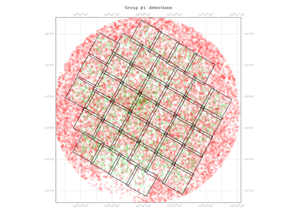
Bad fgroups plots
- Example 1: A wide field view obtained with a photo-lens. Only part of the image (green) is matched with the reference catalogue, due to distortions. Increase the CROSSID_RADIUS.
- Example 2: Total failure. Reason: very small field of view, insufficient sources in the image catalogs. Try lowering the detection thresholds and set distort=1 because not enough sources are available to determine many distortion coefficients.
- Example 3: Inaccurate CD matrix (wrong position angles and/or pixel scale). Try increasing POSANGLE_MAXERR and PIXSCALE_MAXERR. RA and DEC in the FITS header could also be way off. Try increasing POSITION_MAXERR.
- Example 4: LBC_RED@LBT (the red camera at the Large Binocular Telescope, with a quadratic distortion polynomial). Note that only parts of the detectors are matched properly to the sky. Compare to example 5 above.
- Example 5: A wide field of view of a milky way area. While the depth of the reference catalog was ok (about 200 sources returned) the object catalogs contained 10000+ sources per exposure. Increase the object detection threshold DT from e.g. 5 to 50 would bring the source density down to a reasonable level.
- Example 6: That’s a tricky one, based on MOSAIC-II@CTIO. Note that almost all frames are registered nicely. However, the rightmost exposure shows no green matches (only visible at the rightmost edge; the coadded image would be clearly corrupted, though). Reason here was that the WCS information in the FITS header of this single exposure was 7’ offset, whereas the others were all within about 1’. Increasing POSITION_MAXERR to 8’ solved the problem instantly, after many days of trouble shooting on the user side. Mostly problems with scamp have very easy solutions, directly in front of your nose. Lesson: Even modern telescopes mess with you every now and then (not the first time I have seen this; WFC@INT sometimes has had its headers off by 20’).
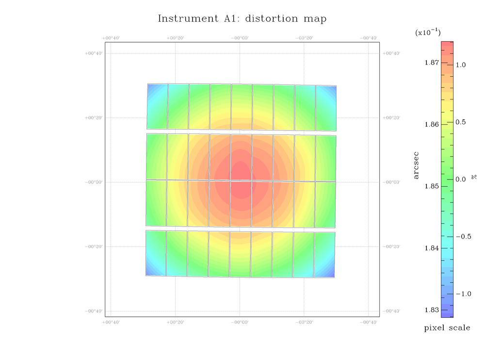
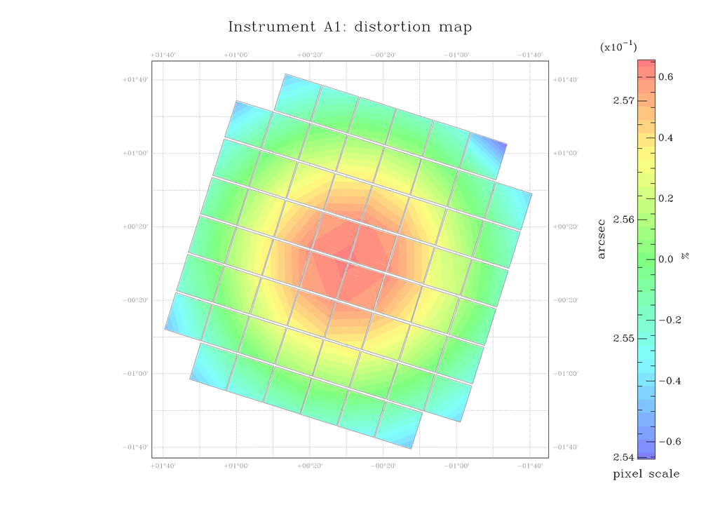
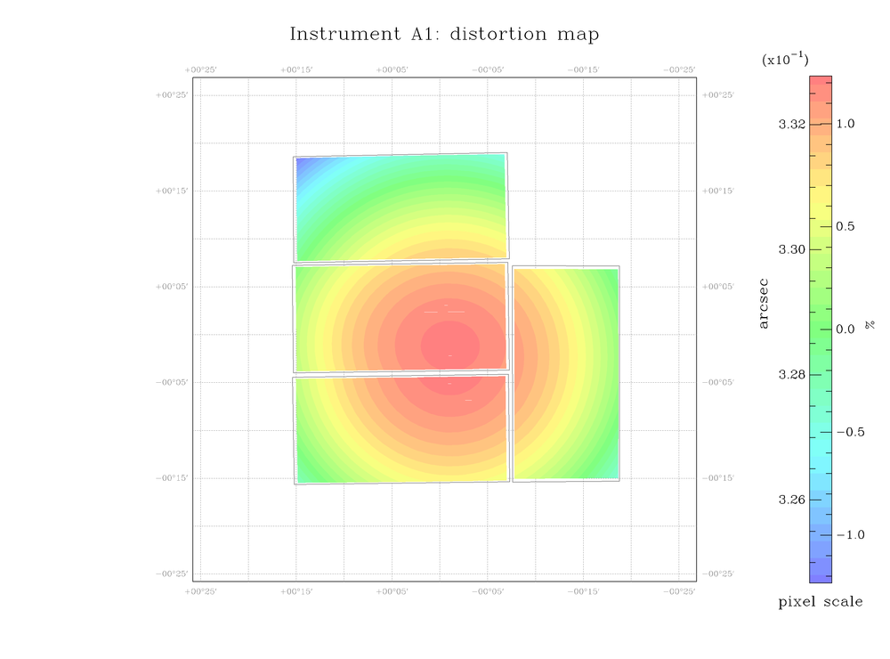
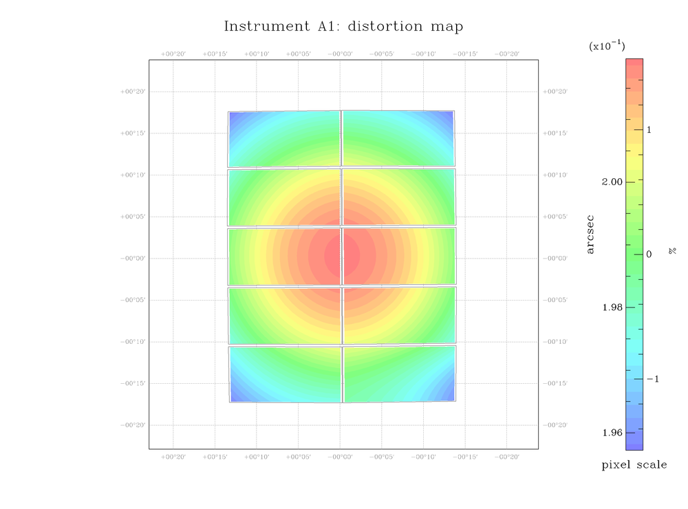
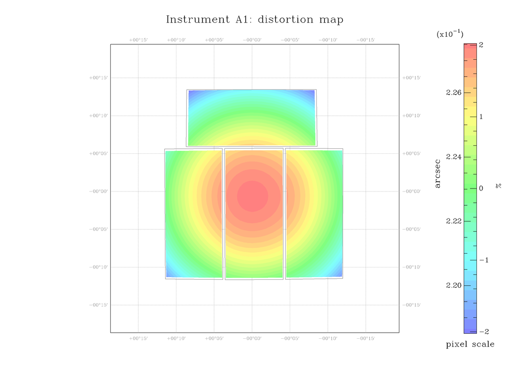
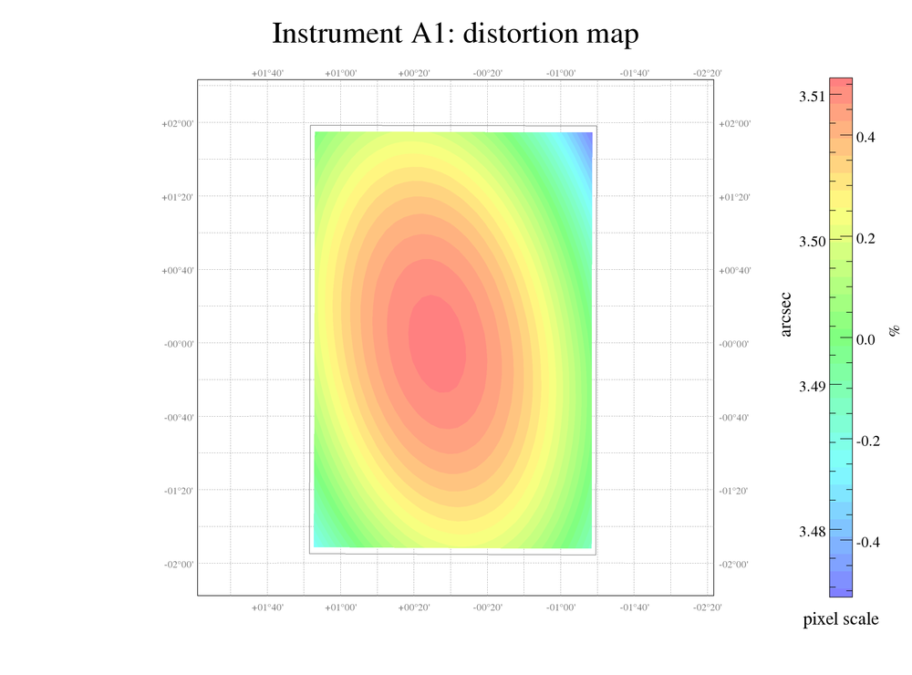
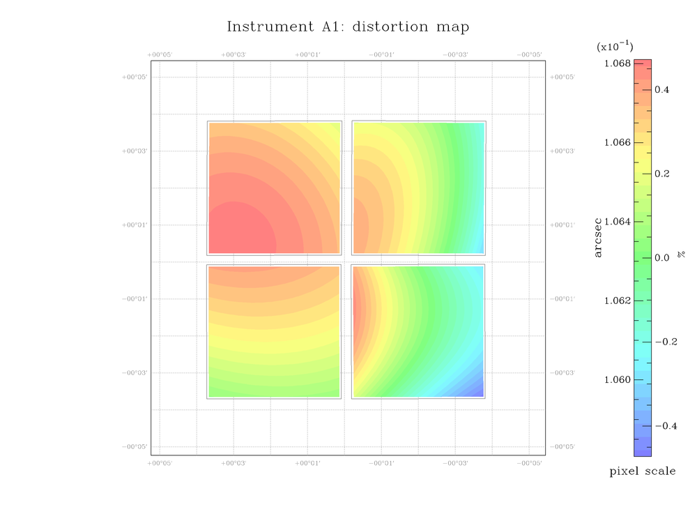
Image distortion: distort
Distortion can be displayed as a variation of the pixel scale across the detector area. Make sure these plots look as symmetric as possible.
Good distort examples
- Example 1: Megacam@CFHT. Note the slight irregularity in the upper half of the image centre. One can do better than that, however this distortion model did not lead to any visible ill effects in the coadded image.
- Example 2: Pan-STARRS. Due to the very short exposure time (30s) and the high galactic latitude only very few sources were visible in this field. Hence only a linear distortion model could be fit to the data. A quadratic fit looked smoother, but showed artifacts with similarly large deviations from reality.
- Example 3: WFC@INT. Note the slight mismatch between the two detectors at the lower left.
- Example 4: WFC@INT. Same as example 3, but using more objects in the reference and the source catalogs.
- Example 5: WFI@MPGESO. The wide-field imager at the 2.2m MPG/ESO telescope is one of the very few instruments where the largest pixel scale does not coincide with the optical axis. You can model it with distort=3, but a higher order model (distort=4..5) (shown: distort=5) yields better results as the curvature of the “ring” is better reproduced.
- Example 6: SuprimeCam@SUBARU
- Example 7: LBC_RED@LBT
Bad distort examples
- Example 1: A wide-field exposure through a photo-lens. Try increasing the number densities in the catalogs or CROSSID_RADIUS to obtain a more concentric pattern.
- Example 2: Pan-STARRS. Note how the chip at the upper right is completely off. It contained only very few sources due to excessive masking. The corresponding images from this chip were removed by hand, then astrometry was repeated.
- Example 3: Megacam@CFHT. Try e.g. to increase the overlap between object catalogs and the reference catalog.
- Example 4: HAWKI@VLT. This is based on a sparse field. Adding another, neighbouring, sparse field fixed the problem. Wide dither pattern patterns or independent data fields help.
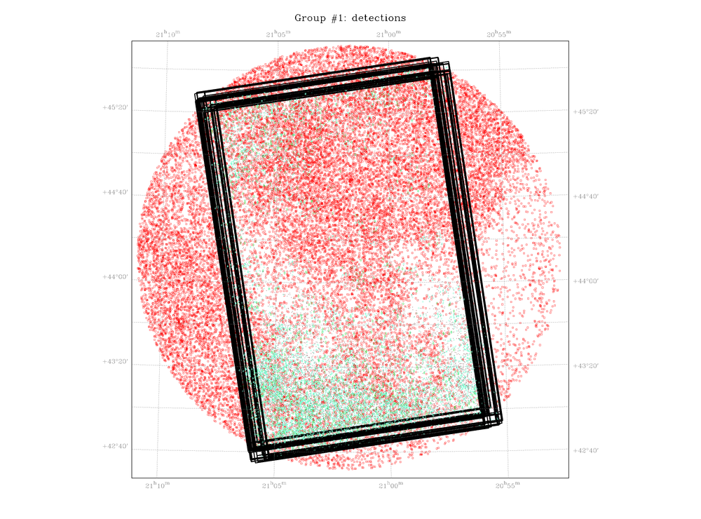
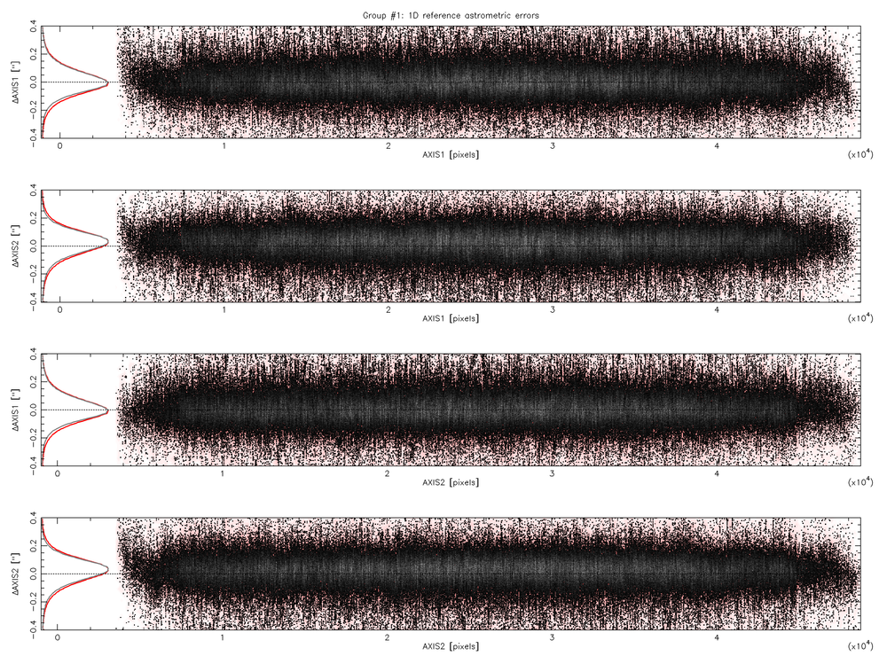
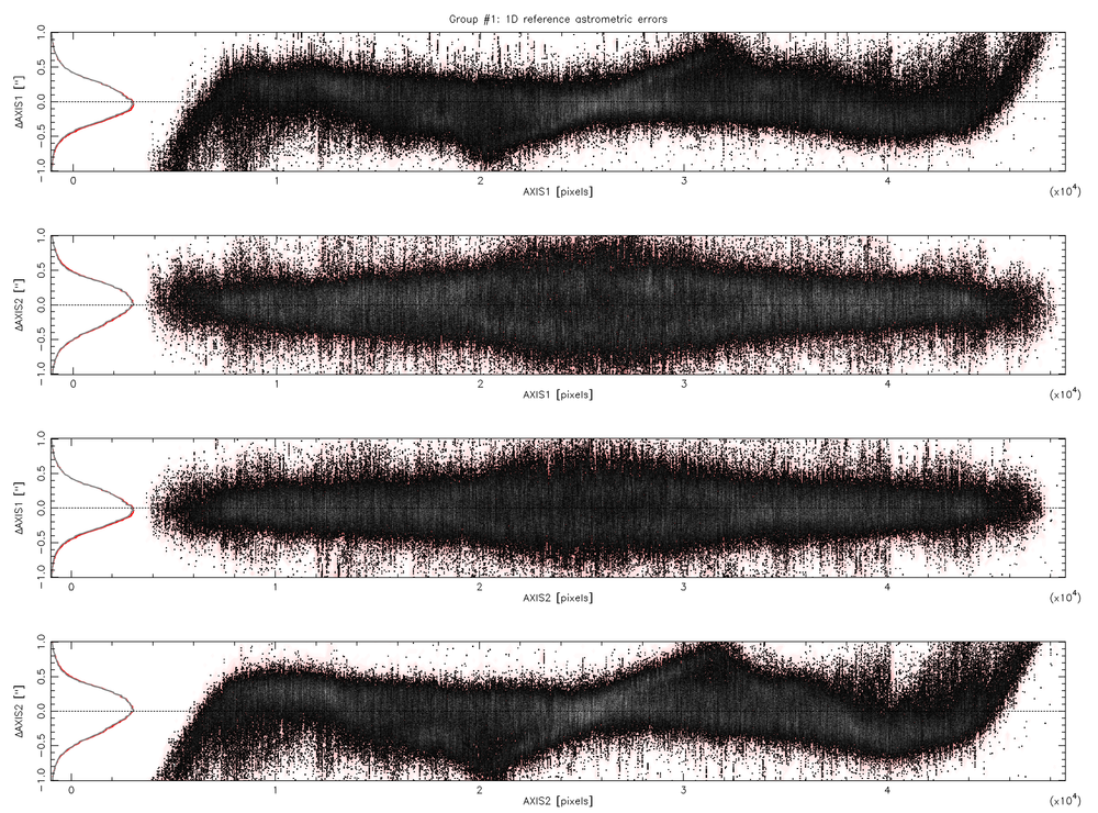
External astrometric residuals: astr_referror1d
Astrometric residuals with respect to the reference catalogue after a solution was found. You’d expect a tight and featureless horizontal distribution whose width is solely determined by the precision of the reference catalog.
Good astr_referror1d examples
- Example 1: Megacam@CFHT, USNO-B1
- Example 2: Pan-STARRS. Note the slight deviations at the outermost edges. Those chips are largely masked and were difficult to match.
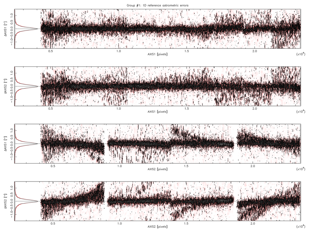
Bad astr_referror1d examples
- Example 1: Megacam@CFHT. Adjust the reference and object catalog settings, or try a different reference catalogue.
- Example 2: Pan-STARRS. The only trick that helped here was putting a lot more weight onto the reference catalogue, ASTREF_WEIGHT=10. Normally this should be avoided as the images have better resolution and higher object density than the reference catalogue. In this case the reference catalogue was SDSS and significantly deeper than these 30s exposures, hence increasing the weight for the reference catalog is justified.
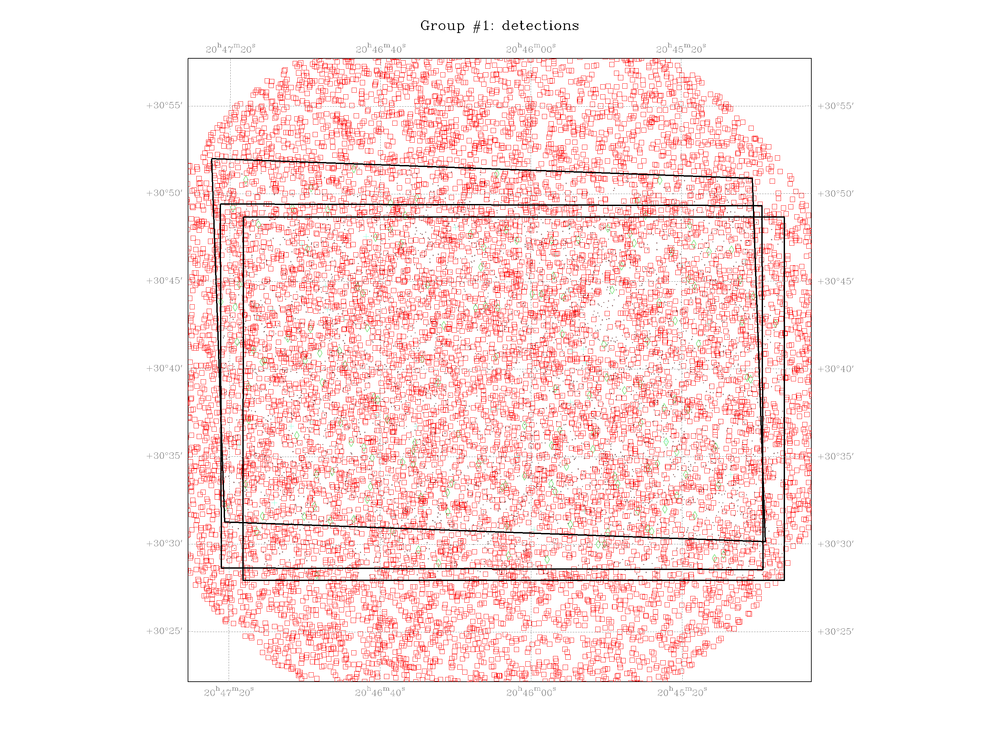
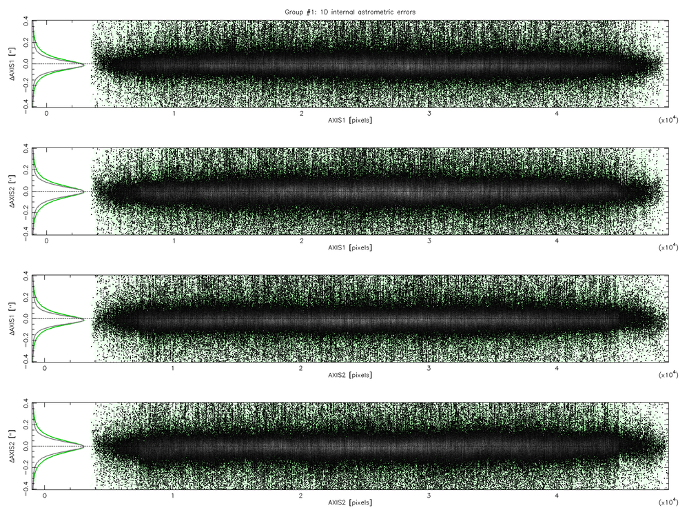
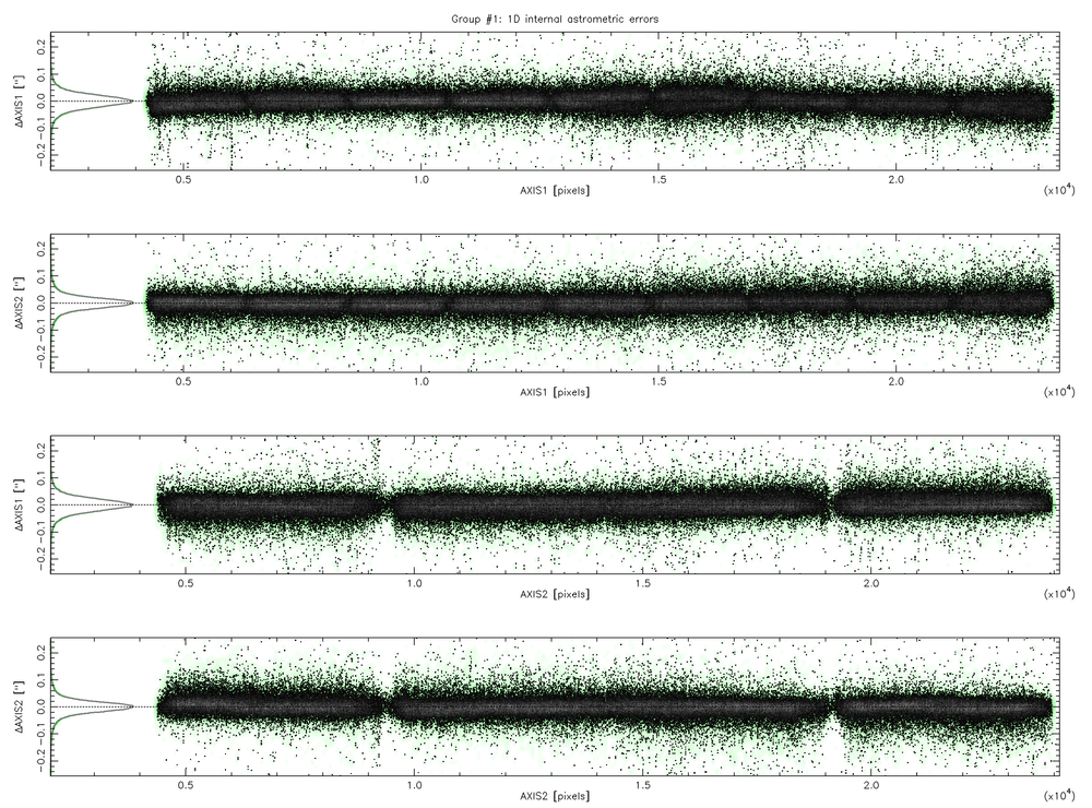
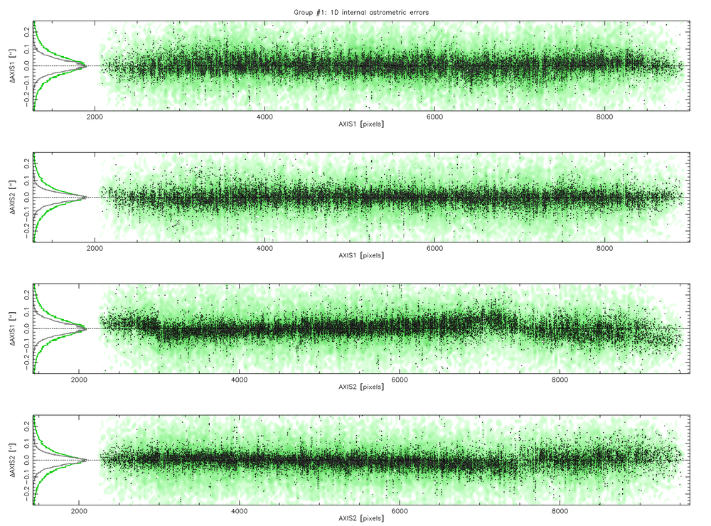
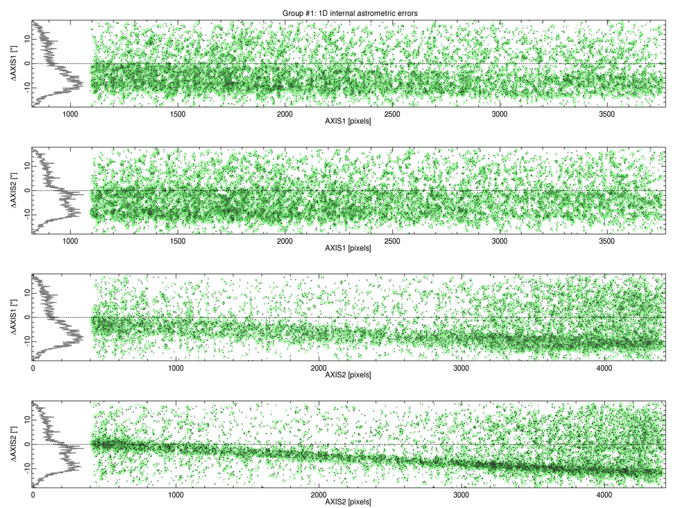
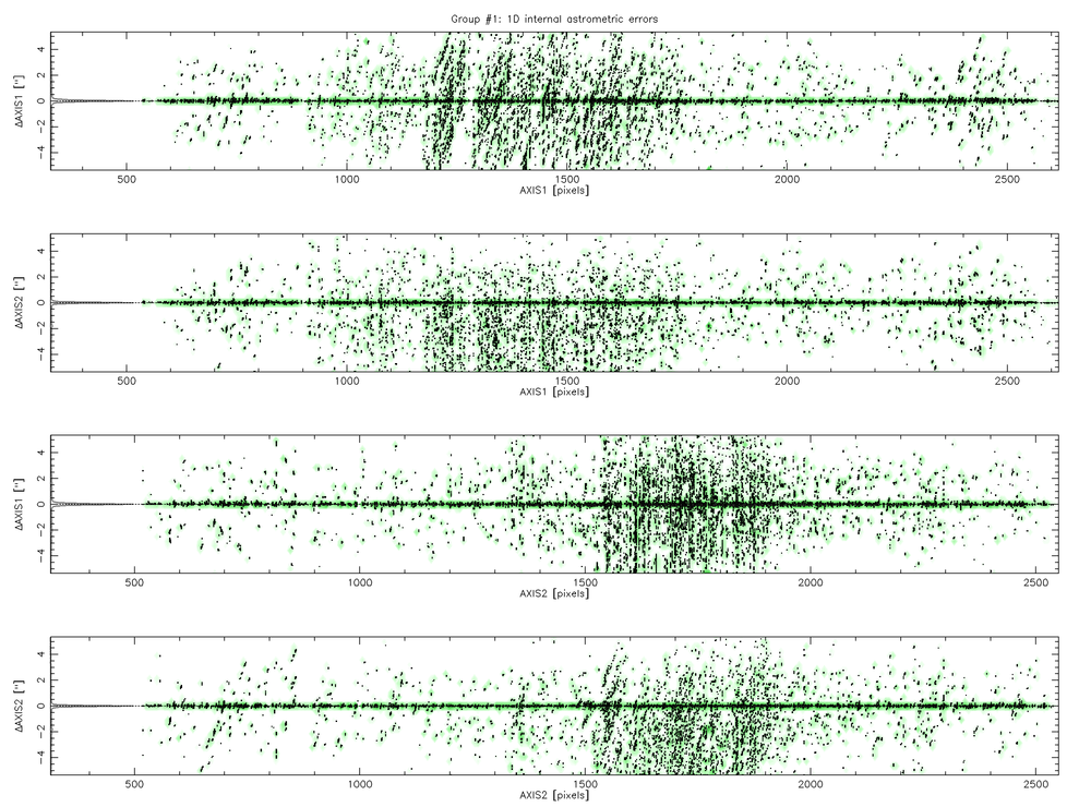
Internal astrometric residuals: astr_interror1d
Astrometric residuals between the individual exposures after a solution was found. You’d expect a tight and featureless horizontal distribution whose width should be on the order of 1/5th-1/20th of a pixel.
Good astr_interror1d examples
- Example 1: Pan-STARRS
- Example 2: Good residuals for a one-chip camera (pixel scale 0.85 arcsec/pixel)
Bad astr_interror1d examples
- Example 1: Megacam@CFHT. Note the small bifurcation in the upper line. The rest is ok.
- Example 2: WFI@MPGESO. The magnitude limit for the reference reference catalog was not deep enough in this case, resulting in badly matched chips.
- Example 3: Note the huge range (10 arcsec) of the y-axis. Normally the range should be about one pixel. Reason here was that the reference catalog downloaded had no overlap at all with the data.
- Example 4: FORS2@VLT observations of a globular cluster. The match is generally good (very tight horizontal line), but there are obvious mis-identifications within the very crowded globular cluster. Repeat the object catalogs with e.g. DEBLEND_MINCONT = 0.01, and try 2MASS instead of USNO-B1. 2MASS has significantly better resolution in crowded objects than USNO-B1 which features many blended or otherwise inaccurate sources in such cases.