If you ever tried to render a nice-looking three-colour picture out of CCD images, you will have noticed that this is far from trivial. The main difficulties are:
THELI does not go all the way to a final image. However, it can prepare suitable scaled images that can be readily processed in third-party software without much further processing.

The first step that has to be done is to select those stacked images that should be combined for a colour picture. THELI assumes that all necessary coadd_xxx directories can be found in the same SCIENCE directory. If you followed the guidelines for processing multi-colour data sets, then this will be the case.
All processing takes place in a new sub-directory
SCIENCE/color_theli/
If this directory already exists, it will be unambiguously renamed into
SCIENCE/color_theli_backup_<timestamp>
SCIENCE dir: Upon opening this dialog, THELI will fill in the currently processed SCIENCE directory. You can change to any other directory you want. If coadditions are present, then these will be shown in the Select coadditions list.
Select coadditions: Mark the coadditons you want to use for the colour image. Several entries can be highlighted at the same time.
Get coadded images: Upon clicking here, THELI will link the coadded images selected into
SCIENCE/color_theli/
If a coadditon was labelled coadd_xxx, the corresponding image and its weight will appear as
SCIENCE/color_theli/xxx.fits
SCIENCE/color_theli/xxx.weight.fits
Once all images are linked, an automatic cropping process kicks in that trims all images such that they have precisely the same size, and such that a particular object will have identical pixel coordinates in all channels. Once this is done, the images will be called
SCIENCE/color_theli/xxx_cropped.fits
SCIENCE/color_theli/xxx_cropped.weight.fits
Note
This works only if the coadditions were created with identical reference coordinates! This step does not involve any resampling anymore as the images already have identical astrometric projections (if the coadditions were done with identical reference coordinates).
Optionally, you can remove some of the cropped images from the list (they will not be deleted from the hard disk, just ignored), or the full list can be restored. The latter is useful if you want to resume work in an already existing color_theli sub-directory.
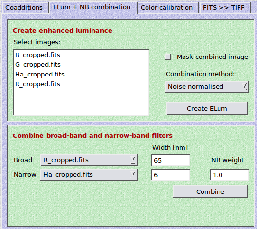
If you took red, green and blue exposures, you will obtain a significantly better (deeper) colour image if you combine the three exposures into a synthetic luminance image.
If you have an unfiltered (clear filter, luminance filter) coadded image, you can add the filtered exposures to it to get even greater depth. However, this will only yield an improvement if
Mask combined image
Pixels which are not covered by all exposures (as judged from the individual weight maps) will be set to zero in the combined image.
Combination method
The following two options are available:
Noise normalised: The background noise of the individual images will be measured in the statistics region specified previously. Images are normalised with respect to their noise and then added (this is similar to the chi-square sense). In this way images with lower background noise contribute more than those with higher noise. The result is called
SCIENCE/color_theli/elum_chisquare.fits
You need to be careful, though. For example, at a dark sky location the background increases significantly from blue to red to unfiltered exposures. If you noise-normalise such data, it can happen that the blue exposure which might carry comparably little signal starts dominating the other exposures, in particular the deep luminance channel.
Mean: The average of the images is calculated. The result is called
SCIENCE/color_theli/elum_mean.fits
If you want to combine plain red-, green- and blue-filtered images, then this is the best approach as it mimics what a luminance filter would have seen.
Note that if you set PHOTINSTRU_KEY = FILTER during astrometry, objects in the three channels will have the same average brightness. If one of them was taken under bad transparency conditions, it will be up-scaled which increases its noise, and can therefore lead to inferior results. Same if you use an image which very low signal-to-noise ratio as compared to the others.
A problem commonly encountered when creating colour pictures is how to include narrow-band exposures in a set of broad-band exposures. This enhances emission line structures, but commonly results in distorted stellar colours or a skewed general appearance of the image. The solution is straight-forward, and since it has not been documented anywhere else for amateur astronomers, I present it in sufficient detail so that it can be reproduced with other software.
Consider two coadded R-band and  images. Both cover the
line and shall fully transmit it. Two requirements have
to be met:
images. Both cover the
line and shall fully transmit it. Two requirements have
to be met:
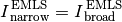
Problem: Let’s consider stars only, which are continuum emitters. When adding the narrow-band exposure to the broad-band exposure, we make the stars brighter, and hence change the colour balance with respect to the other broad-band filters.
Solution: We have to first downscale the broad-band image by some amount, so that the final stellar flux emerges unchanged once the narrow-band image is added.
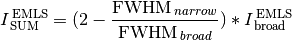
The scaling factor is easily calculated from the filters’ FWHM ratio. For example, if the narrow-band filter transmits 10% of the broad-band filter, then we have to scale the broad-band image by a factor of 0.9 to accomodate the additional narrow-band flux. Therefore,
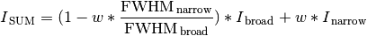
Here,  and
and  represent the two images,
and
represent the two images,
and  is a weighting factor that is 1 by default. Now lets consider how this formula
works for continuum and emission line sources.
is a weighting factor that is 1 by default. Now lets consider how this formula
works for continuum and emission line sources.
Continuum source (star): We assume that the star has a flat spectrum within the bandpasses, which is a good enough approximation for our purposes. Seen through the narrow-band filter, the star then has a flux of
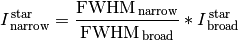
Insert this for in the first equation, and you will find that
Therefore, a star’s brightness is conserved in the combined image.
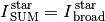
Emission line source: Both the R-band and the filter encompass the
emission line and (nearly) fully transmit it. This means that a pure
emission line source, which does not emit outside the narrow bandpass, will appear
equally bright in both filters:
Insert this for in the first equation, and you will find that for a
weighting factor of  we have
In our example, where the filter has 10% the width of the
broad-band filter, this means that the flux is enhanced by
a factor of 1.9 compared to the broad-band image, while maintaining stellar fluxes.
This is sufficient for most purposes. For weighting factors of  or
or  , the enhancement factor would then be 2.8 and 3.7, respectively.
This method works for all sets of narrow- and broad-band filters that cover the same emission line, e.g. a blue or green filter and the [OIII] doublet. If the broad-band filter transmits the emission line to e.g. only 60%, because the line is at the edge of the bandpass, then this can easily be corrected for by multiplying the FWHM ratio by 0.6.
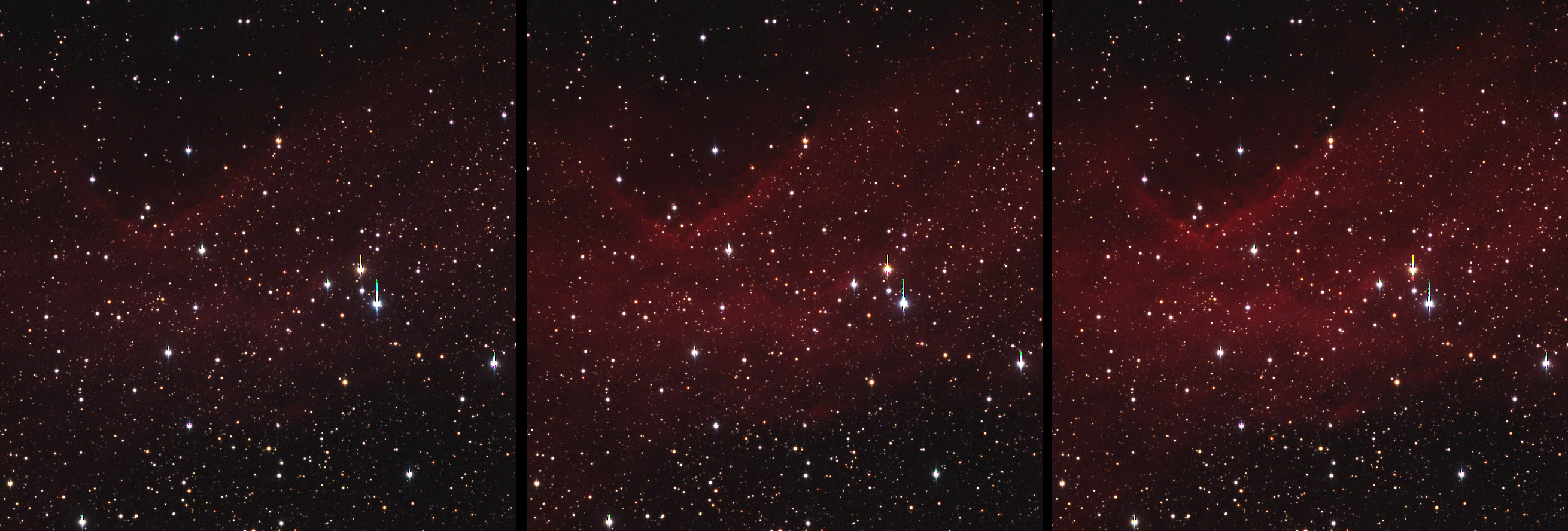
NGC 7822: Left: RGB; Middle: (RHa)GB,  ; Right: (RHa)GB,
  ;
;
Note that the stars’ colours remain unchanged, while the extended nebulosity gets increasingly
enhanced with growing weight factors. Exposure data: ST10XME, 102mm FSQ, RGB = (8x8x8)*240s,
= 6*1800s. Apart from identical contrast stretching no further image
processing took place for these three images. Colour calibration was achieved based on BVR
magnitudes of 50 stellar NOMAD sources (see next section below).
The idea behind colour calibration is to have a solar-type G2V star appearing white in the colour picture. If this only depended on the total telescope throughput (mirror reflectivity, corrector lenses, filter transmission and quantum efficiency), fixed calibration factors could be used. However, the atmosphere changes its transparency continuously, either because of changing airmass, dust, cirrus, humidity etc. Atmospheric extinction has a significant impact even in very clear nights when targets are rising or setting, affecting the calibration factors by 10% or more. If exposures are taken in different nights, the balance can be off even more. Variations on the level of a few percent are easily seen by the eye in a colour picture.
The best way to obtain the colour calibration is to identify solar-type stars directly in the images. Like that
However,
To work around these problems, one can drop the requirement of selecting known G2 stars as standards, and take G2-alike stars instead. These can be selected photometrically from an external reference catalogue by means of their colour indices. In the classic Johnson-Cousins UBVRI system, G2 stars have on average B-V = 0.65 and V-R = 0.5. In SDSS ugriz filters we have u-g = 1.43 and g-r = 0.44. Once a sample of suitable field stars is known, they can be identified in the images and calibration factors are readily determined.
What if no G2-alike stars are found, i.e. in under-dense regions or in images with a very small field of view? In this situation a good white point can still be obtained by making all stars on average white. Compared to the PCC method the blue and green channels appear enhanced. The reason is that the average stellar population is somewhat reddish (80% of all main sequence stars in the solar neighbourhood are red dwarfs).
The calibration factors will also depend on the line of sight: stars in the galactic halo have different characteristics than those in the disk, and towards the galactic bulge things change once more. Thus, one will obtain slightly different calibration factors depending whether one looks outside the disk, into the disk, or towards the galactic centre. Galactic extinction (interstellar reddening) will be partially removed by this method, which might be a desirable effect (or not).
THELI offers both the PCC method as well as the average white approach.
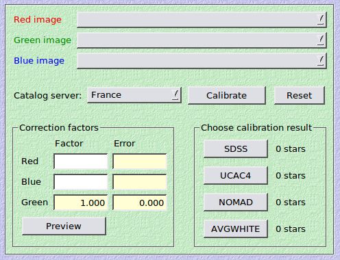
Calibration is fairly easy:

The last step is to convert the FITS images to 16-bit TIFF format. The latter can be exported into e.g. Photoshop or other programmes for further processing. Note that for Photoshop FITS Liberator is available, which can directly import the FITS images. The next release of FITS Liberator will be a stand-alone tool that does not require Photoshop anymore.
Before you can proceed in Photoshop or with FITS Liberator, you must fine-tune the sky background and apply the colour calibration factors:
Click on Get statistics, which will measure the mean background level and its rms in the statistics section defined previously.
Then choose between two methods to create the 16-bit TIFF images:
This will convert each FITS image to a stand-alone TIFF image, which you have to combine in an external programme to render the final colour image. You can manually override THELI’s suggestions:
TIFFmin: This will be the black-level of the TIFF image, i.e. all pixels in the FITS image with values below this threshold will be represented as black in the 16-bit TIFF. THELI identifies the image with the largest background noise and multiplies this value with -6. The resulting value, TIFFmin, will be the same for all exposures. In this way the sky background is not clipped. Usually you can leave this value unchanged.
TIFFmax: This is the white-level of the TIFF image, i.e. all pixels in the FITS image with values above this threshold will be represented as white in the 16-bit TIFF. TIFFmax is set arbitrarily 500 times higher than TIFFmin.
If you want to display even brighter image parts without saturation, increase this value, otherwise leave it (or decrease it). For example, you observed a galaxy with a bright core and don’t want this core to be saturated. Measure its brightness in the three colour channels (e.g. red=25, green=15, blue=12) and set TIFFmax to a value that is somewhat higher than the maximum of the three (e.g. to 30).
Warning
TIFFmin and TIFFmax must be identical for the red, green and blue channel, otherwise the colour calibration performed previously will be distorted. You may choose different values for luminance channels.
Using the Convert FITS to TIFF button will convert all images listed in the statistics table into TIFF images:
SCIENCE/color_theli/*.tif
If you want to use the corresponding FITS images (colour calibrated and sky subtracted) for e.g. FITS Liberator, use
SCIENCE/color_theli/*_2tiff.fits
A slightly different approach uses the STIFF package. STIFF creates individual 16-bit TIFF images as well, but can also combine the three colour channels into a colour TIFF, such that you don’t have to do this in external software anymore. In addition, STIFF offers to increase the colour saturation and to apply a non-linear gamma correction. However, these things can also be done in any classic image processing software).
STIFF parameters
Note
STIFF applies the sky background values listed in the statistics table, the same as used by the classic FITS to TIFF conversion.
Min | max level: Same as TIFFmin and TIFFmax described above.
Saturation: Only meaningful when creating a RGB colour TIFF
Gamma: Non-linear gamma correction to the dynamic range.
Make RGB image: Select here which images should be converted. If you choose Make RGB image, the red, green and blue images defined in the colour calibration section will be converted into a 3-colour RGB TIFF image, saved as
SCIENCE/color_theli/rgb_stiff.tif
If you want to convert a specific channel into a grey-level TIFF, then just select it from this pull-down menu. The resulting TIFF image will be displayed automatically and is stored as
SCIENCE/color_theli/*_stiff.tif
Only one TIFF at a time will be created when clicking on Convert FITS to TIFF.