Next: Microphysical Processes Up: Photo-ionisation and Recombination Previous: Photo-ionisation without recombinations
| (2.9) |
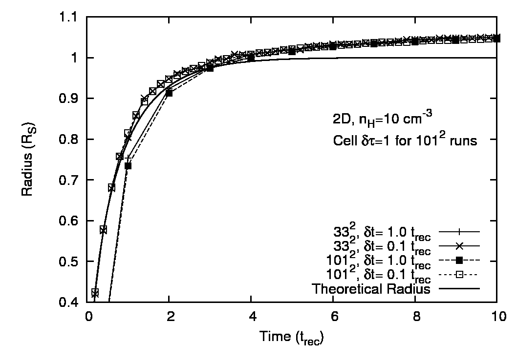
Fig. 2.14 shows the position of the I-front as
a function of time for simulations with recombinations included, with
the analytic solutions plotted as a solid line. Note that for the low
density runs the cell optical depth is
![]() and so the
I-front is resolved. In this case the analytic approximation of a
sharp I-front breaks down and the final radius deviates from
and so the
I-front is resolved. In this case the analytic approximation of a
sharp I-front breaks down and the final radius deviates from ![]() .
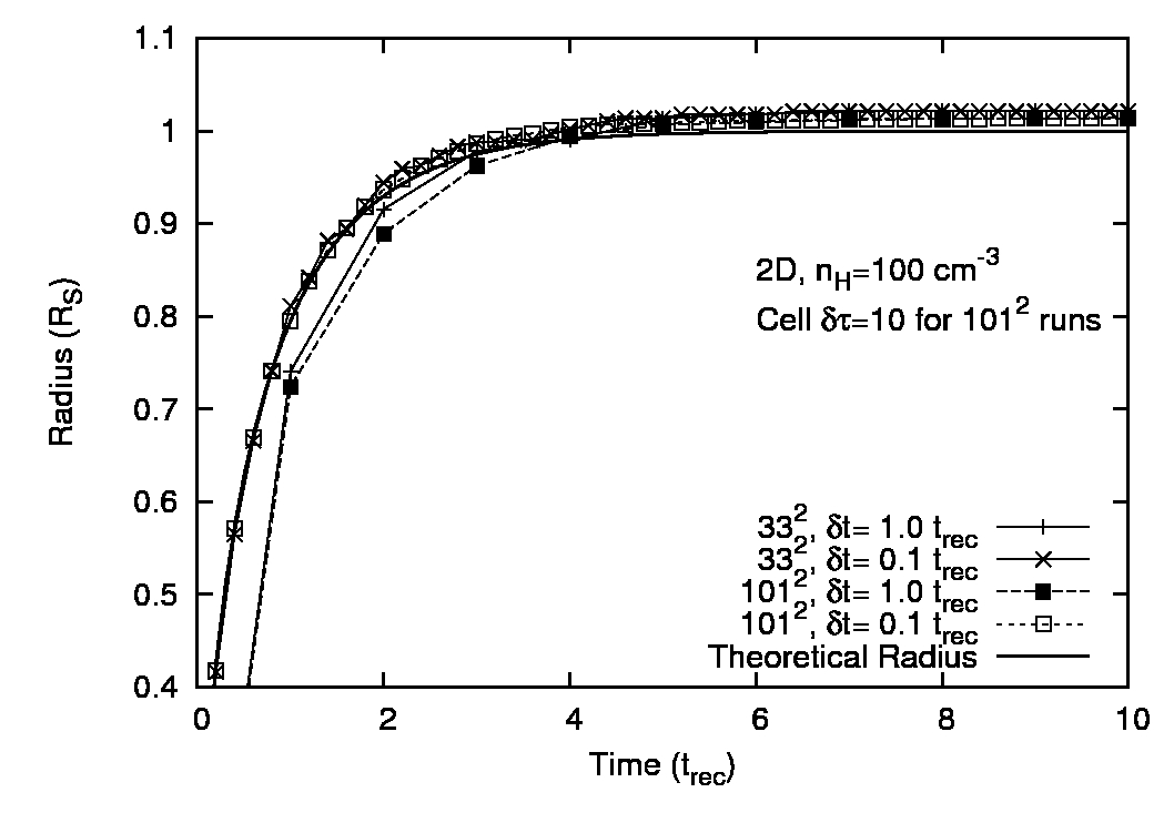
For the higher density runs the I-front is unresolved and its mean
position is always within
.
For the higher density runs the I-front is unresolved and its mean
position is always within ![]() per cent of the analytic value except
at very early times when it has only crossed a few cells, or when the
timesteps are of order the recombination time. This is an expected
limitation of the C
per cent of the analytic value except
at very early times when it has only crossed a few cells, or when the
timesteps are of order the recombination time. This is an expected
limitation of the C![]() -ray method since it uses time-averages of the
photon flux through each cell (see Mellema, 2006). For the
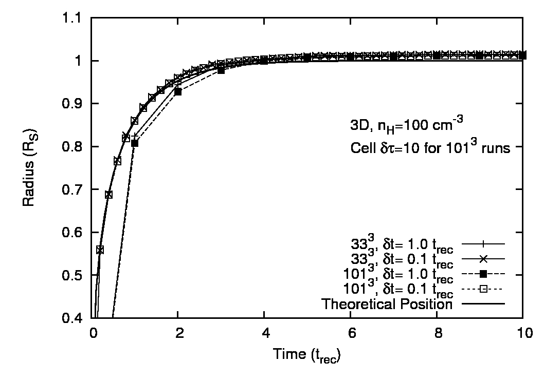
tests where
-ray method since it uses time-averages of the
photon flux through each cell (see Mellema, 2006). For the
tests where
![]() we underestimate the I-front
velocity while it expands to
we underestimate the I-front
velocity while it expands to ![]() . The error is
slightly larger at higher spatial resolution because we have to do the
same inaccurate time-average across more cells and the error is always
on the side of losing photons. For sufficient time resolution,
however, the I-front propagates at the correct speed, and it is worth
noting that the photo-ionisation time for a cell is much shorter than
the recombination time while the I-front is expanding rapidly. We do
not need to resolve this timescale to get accurate results. This is
the major strength of the C
. The error is
slightly larger at higher spatial resolution because we have to do the
same inaccurate time-average across more cells and the error is always
on the side of losing photons. For sufficient time resolution,
however, the I-front propagates at the correct speed, and it is worth
noting that the photo-ionisation time for a cell is much shorter than
the recombination time while the I-front is expanding rapidly. We do
not need to resolve this timescale to get accurate results. This is
the major strength of the C![]() -ray algorithm.
-ray algorithm.

 |