Photo-ionisation and Recombination

Photo-ionisation was tested in conjunction with raytracing using similar tests to those in Mellema (2006), where the dynamics is switched off. In 1D, when we have no recombinations and a source off the domain in one direction, an I-front just moves with constant speed equal to the flux of photons divided by the number density of neutral atoms:

$$R_{if}(t) = R_{if}(0)+\frac{F_{\gamma}}{n_{\mathrm{H}}}(t-t_0)\;,$$ (2.3)

where $F_{\gamma}$ is the photon flux in units of $\,$cm$^{-2}\,$s$^{-1}$. With recombinations, the I-front gradually slows until it reaches a limiting position where the incident flux is just sufficient to re-ionise all the ions that are recombining. The solution in this case is

$$R_{if}(t) = \frac{F_{\gamma}}{\alpha_{rr}n_{\mathrm{H}}^2}[1-\exp(-\alpha_{rr}n_{\mathrm{H}}t)] \;,$$ (2.4)

where the initial velocity is $F_{\gamma}/n_{\mathrm{H}}$ and the recombination time is $t_{rec}=1/(\alpha_{rr}n_{\mathrm{H}})$. Here $\alpha_{rr}$ is the (case B) Hydrogen radiative recombination coefficient set to a constant for these test problems ( $\alpha_{rr}=2.59\times10^{-13}\,\mathrm{cm}^{3}\,\mathrm{s}^{-1}$), and $n_{\mathrm{H}}$ is the Hydrogen number density.

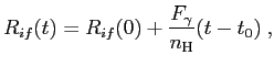
For 2D we put a source at the centre of the grid. We have slab symmetry, so really we have an infinite line source of photons, emitting at a rate $\dot{n}_{\gamma}$ per second per unit length. The quivalent results are: for no recombinations

$$R_{IF}(t) =\sqrt{\frac{\dot{n}_{\gamma}t}{n_{\mathrm{H}} \pi}} \;,$$ (2.5)

and with recombinations

$$R_{IF}(t) = \sqrt{\frac{\dot{n}_{\gamma}}{n_{\mathrm{H}}^2\alpha_{rr} \pi} [1-\exp(-n_{\mathrm{H}}\alpha_{rr} t)]} \;.$$ (2.6)

In 3D the equivalent results are

$$R_{IF}(t) = \sqrt[3]{\frac{3\dot{n}_{\gamma}t}{4\pi n_{\mathrm{H}}}} \;,$$ (2.7)

and

$$R_{IF}(t) = \sqrt[3]{\frac{3\dot{n}_{\gamma}}{4\pi n_{\mathrm{H}}^2\alpha_{rr}} [1-\exp(-n_{\mathrm{H}}\alpha_{rr}t)]} \;.$$ (2.8)

The simulations without recombinations will hence expand forever, but with recombinations we should reach a fixed radius in (effectively) finite time due to the exponential relaxation. After 3-5 recombination times we should be very close to the Strömgren radius.

We first tested with 1D rays from a source at infinity, without dynamics or recombinations. For a grid with 1000 cells, we computed models with cell optical depths $\delta\tau=\{0.1,1,10,100\}$, and where the total number of timesteps varied from $t_{\mathrm{sim}}/\delta t = \{10^1,10^2,10^3,10^4\}$. The error in I-front position compared to the analytic value was found to converge rapidly to less than one cell width with increasing time resolution. For models with recombinations turned on, errors were no more than than one cell width for all runs with $>10$ timesteps per recombination time, except for low density models where the I-front is resolved.

In 2D and 3D, we computed the expansion of circular and spherical I-fronts from a point source into a static medium, with and without recombinations. Without recombinations, the models provide a test of photon conservation (by comparing the number of ions to photons emitted as a function of time). With recombinations we model the expansion of an I-front to the Strömgren radius, $R_{s}$, testing both the expansion velocity and the final radius against a known analytic solution.