Photo-ionisation without recombinations

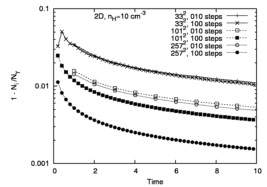
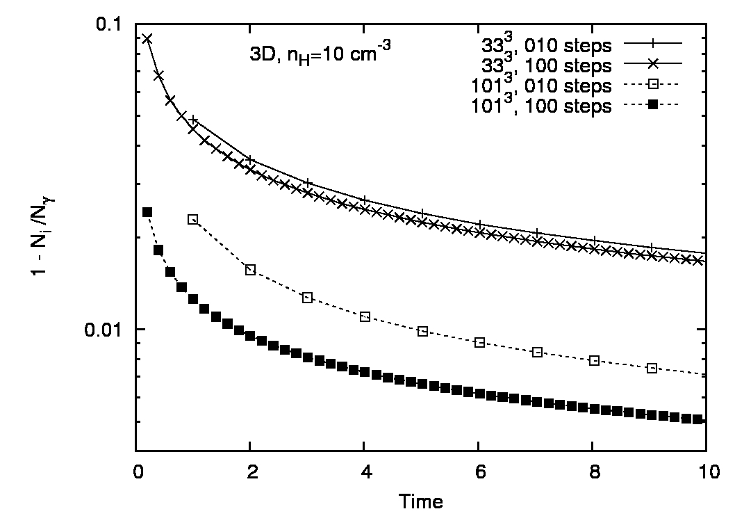
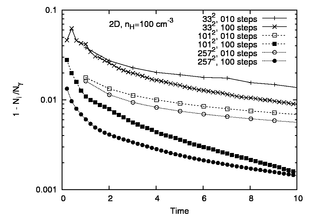
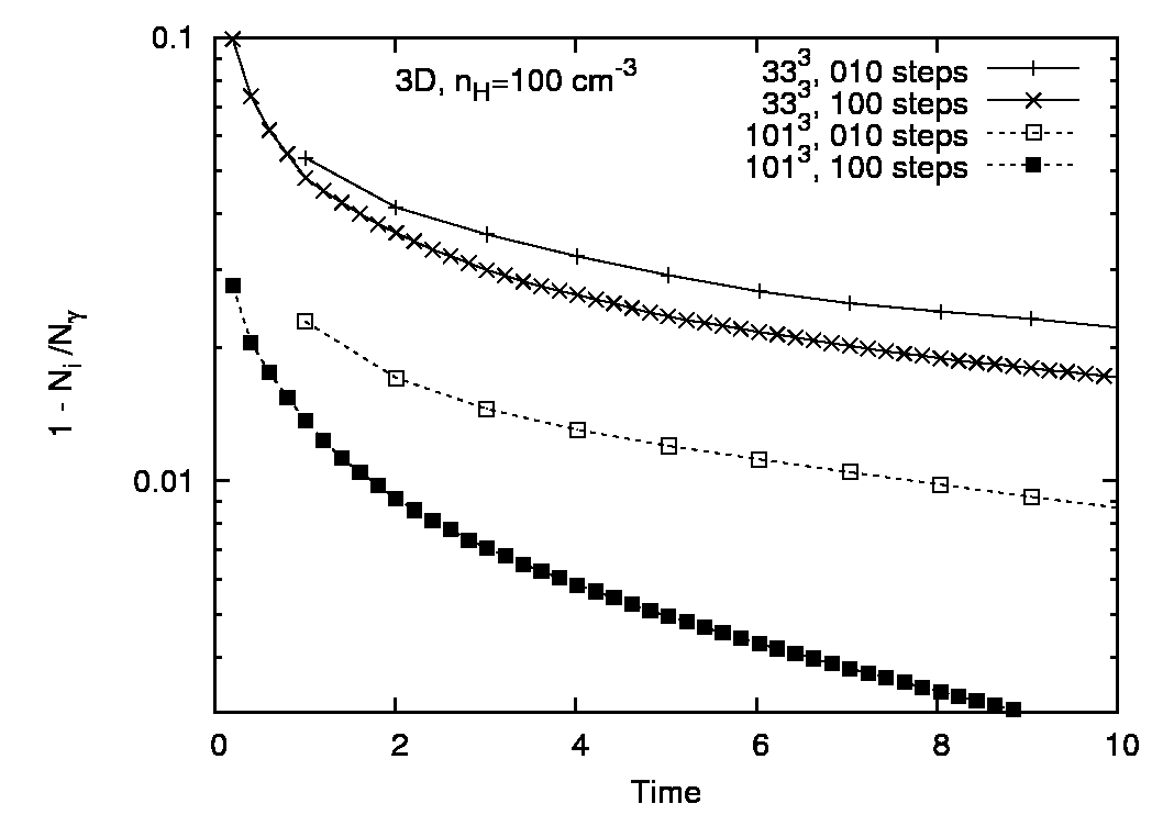
We plot the photon conservation in Fig. 2.13, for 2D on the left and 3D on the right. These figures show the relative sizes of ray-tracing and time-integration errors as a function of resolution and dimensionality. For the very low resolution runs ($33^2$ and $33^3$ cells) we lose between 1 and 10 per cent of photons due to interpolation errors in the ray-tracing when the ionised region is $<10$ cells across. With increased spatial resolution the errors decrease strongly whereas increased time resolution doesn't help the 33 cell runs significantly. There is a dramatic improvement in accuracy with time resolution for the 101 and 257 cell runs. These results show that the errors are interpolation dominated when the number of cells is much smaller than the number of timesteps and time-integration dominated in the opposite limit.

Using the weighting scheme recommended by Mellema (2006) we find that I-fronts are circular to within a cell width over a wide range of densities, luminosities, and spatial and temporal resolutions.

Figure 2.13: Tests of the radiative transfer algorithm in 2D (left) and 3D (right). The plots compare the number of ions to the number of photons emitted for a source in a uniform medium with dynamics and recombinations switched off. The source is at the centre of the domain, and the I-front remains on the domain for the duration of the simulations. This is a scale-free problem which we have run with parameters such that the cell optical depth is $\delta \tau =1$ (first two panels) or $\delta \tau =10$ (final two panels) for the runs with $101^2$ and $101^3$ cells ( $\delta \tau =[3.06,30.6]$ for lower resolution and $[0.393,3.93]$ for higher resolution). We always lose some photons due to the interpolation, but this decreases dramatically with resolution.