Next: Advection of a Magnetic Up: Multi-dimensional Adiabatic Tests Previous: Rotated Shock Tube Tests
The setup is as follows: the domain is
![]() ,
, ![]() , with
spatial resolutions of
, with
spatial resolutions of
![]() and
and ![]() grid
cells. We use an ideal gas equation of state with
grid
cells. We use an ideal gas equation of state with
![]() and an
undisturbed gas state
and an
undisturbed gas state
![]() . A Mach 10
shock is set up whose initial position on the lower boundary is
. A Mach 10
shock is set up whose initial position on the lower boundary is
![]() and whose propagation direction is
and whose propagation direction is
![]() from the
from the
![]() -axis (moving down onto the reflecting
-axis (moving down onto the reflecting ![]() -axis). Special fixed
boundary conditions are set up for
-axis). Special fixed
boundary conditions are set up for ![]() and
and ![]() allowing the
shock to propagate off the domain. For the upper boundary
allowing the
shock to propagate off the domain. For the upper boundary ![]() a
time-dependent boundary is imposed to allow the shock to propagate
onto the domain as though it extended to infinity.
a
time-dependent boundary is imposed to allow the shock to propagate
onto the domain as though it extended to infinity.
The simulation is run until ![]() , by which time the shocks should
be nearly at the right edge of the domain. For these tests a Courant
(CFL) number
, by which time the shocks should
be nearly at the right edge of the domain. For these tests a Courant
(CFL) number
![]() is used, with viscosity
is used, with viscosity
![]() or
or
![]() .
.

 |


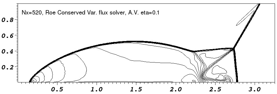 |
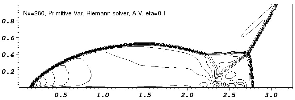
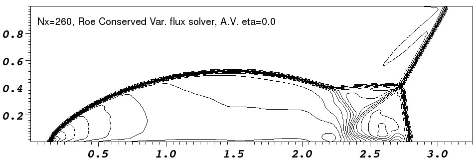
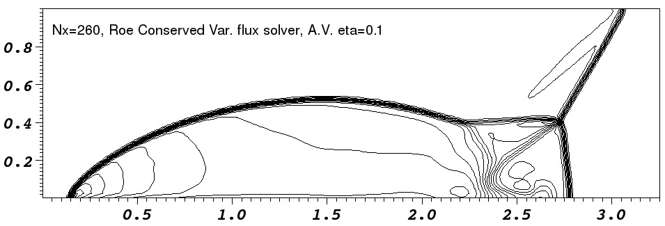
In the low resolution runs, the `jet' near the reflection axis clearly
propagates further in the ![]() -direction in the runs without added
diffusion. This is the well known ``carbuncle'' problem and it is
seen most clearly in the Roe-solver run where the shock is kinked as
it approaches the
-direction in the runs without added
diffusion. This is the well known ``carbuncle'' problem and it is
seen most clearly in the Roe-solver run where the shock is kinked as
it approaches the ![]() axis. The runs with diffusion added do not
have this problem at all, and the flow in other regions is largely
unaffected. In particular the shocks are not much more spread out
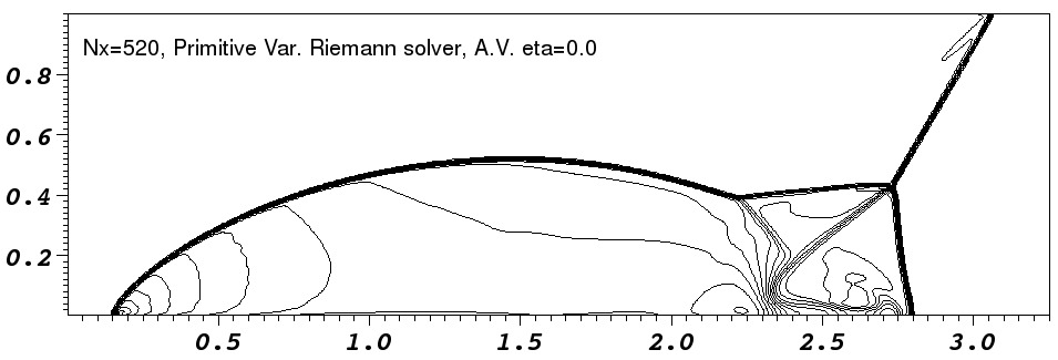
in models with extra diffusion. For the high resolution runs the
shocks and other discontinuities are better resolved, as expected, and
the effects of added diffusion are very similar to lower resolution
runs. Comparison with fig. 16 of Stone (2008) shows that our
code appears slightly more diffusive than Athena. This is
particularly noticeable in the contact discontinuities.
axis. The runs with diffusion added do not
have this problem at all, and the flow in other regions is largely
unaffected. In particular the shocks are not much more spread out
in models with extra diffusion. For the high resolution runs the
shocks and other discontinuities are better resolved, as expected, and
the effects of added diffusion are very similar to lower resolution
runs. Comparison with fig. 16 of Stone (2008) shows that our
code appears slightly more diffusive than Athena. This is
particularly noticeable in the contact discontinuities.
The artefact noticeable behind the shock near ![]() is caused by a
combination of the initial and boundary condition. The initial shock
is perfectly sharp and a low amplitude startup wave is left behind
it (e.g. Falle, 1998). Additionally the boundary condition
has a perfectly sharp shock whereas the time integration smears the
shock over a number of zones. This imperfect coupling of the
artificial boundary shock to the evolving shock on the domain causes a
wave to propagate into the region behind the shock. Having a more
detailed boundary condition would largely remove this feature.
is caused by a
combination of the initial and boundary condition. The initial shock
is perfectly sharp and a low amplitude startup wave is left behind
it (e.g. Falle, 1998). Additionally the boundary condition
has a perfectly sharp shock whereas the time integration smears the
shock over a number of zones. This imperfect coupling of the
artificial boundary shock to the evolving shock on the domain causes a
wave to propagate into the region behind the shock. Having a more
detailed boundary condition would largely remove this feature.