Plotting Visibilities

1. You may tire of all this listing of numbers, and would prefer to make some plots. The task uvplt   provides a variety of choices when plotting visibilities, and ancillary information associated with the visibilities. It has rather a lot of inputs, so read the help file first for the details. We discuss some of the keywords below and then give a couple of examples.
   • vis specifies the visibility datasets to plot. It can take multiple dataset names, each separated by a comma, and wildcard expansion (via an asterisk) of file names is supported.

   • line and select are the standard visibility selection keywords. The default for the line parameter is the first channel, so be careful if you are plotting a dataset with many channels; you would need to explicitly select the channels you require, especially as in multi-channel datasets the first few channels are either rubbish or flagged. The default for select is all the data.

   • Select the desired polarisation or Stokes parameter with stokes. Conversions from linear (or circular) polarisations to Stokes parameters are supported. You can have any combination that you like on one plot, but they will all be plotted with the same symbol. This generally does not matter as any signal will make the distinctions clear and colours are used on devices that support it.

   • axis is used to tell uvplt what to plot on each axis. You can put any of the allowed choices (see the help file) on either of the axes. For example, you could set axis=imag,real to plot the imaginary part of the visibility on the x-axis, and the real part on the y-axis. Such a plot is very useful to examine calibrator data. The default is to plot visibility amplitude versus time.

   • xrange and yrange specify the plot ranges for the x- and y-axes. If they are unset, the plot(s) are auto-scaled. Generally, each of these keywords takes two values. However, if the corresponding axis is time, then you must specify eight values; a day, hour, minute and second for the start and stop times.

   • You can average the plotted quantities in time by setting average in minutes (but see the options keyword for exceptions to this unit). Baselines and polarisations are averaged separately (unless options=avall), but channels are not -- they are all lumped in together.

     The complex visibilities are vector averaged by default, and the real quantities are scalar averaged by default. For example, if you ask for an averaged amplitude or phase, the real and imaginary parts of the visibilities are averaged, and then the amplitude or phase formed. If you ask for, say, u versus time, u is scalar averaged. You can override the vector averaging by setting options=scalar; a scalar averaged amplitude is useful if the phase is winding rapidly. A scalar averaged phase is pretty meaningless under most conditions.

     Averaged points are plotted with filled-in circles rather than dots, unless options=dots.

   • If you plot, say, amplitude or phase versus time, you may find the application of Hanning smoothing useful to knock off the rough edges, rather than applying box-car smoothing (which is what you get when you average in time). Set hann to an odd number.

   • If you do not want to see all the selected points, you can set inc to plot every incth point that would normally have been selected. For example, it is useful for plotting u versus v . Be careful of a value of inc that divides exactly into the number of baselines in time-ordered data (you end up seeing the same baselines over and over).

   • uvplt has a vast complement of options. They are all described in the help file. We will mention a few of them here.

     Like most of the visibility tasks, it has nocal, nopol and nopass to turn off the calibration tables, which, by default, are applied if they exist. MIRIAD will tell you when it applies any calibration table.

     By default, uvplt puts each baseline on a separate sub-plot on the page (see nxy below). Setting options=nobase means that all baselines go on the same plot.

     options=scalar instructs uvplt to do scalar averaging in time.

     On occasion, you may not wish to time average baselines or polarisations separately. Setting options=avall instructs uvplt to average together everything that is to be plotted on a separate sub-plot.

     options=rms instructs uvplt to plot error bars on any time-averaged quantities. However, note that error bars are not yet implemented for vector averaging.

     By default, if you plot many sub-plots (one for each baseline), all the sub-plots are displayed with the same axis ranges, which encompass the data on all the sub-plots. Setting options=xind or options=yind (or both) scales that axis on each sub-plot independently.

     uvplt has an interactive mode invoked by setting options=inter. This gives you a chance to redraw the plot with different axis ranges, without having to read all the data in again. This option also prompts you for a new plot device, so that following display and range refinement on your workstation, you can them make a hard copy without re-running uvplt .

   • Select the PGPLOT device to plot on with a command such as device=/xs (plot on local X-window) or device=amp.plt/ps (write plot to a PostScript file called `amp.plt').

   • Specify the number of sub-plots in the x- and y-directions with a command such as nxy=4,3.

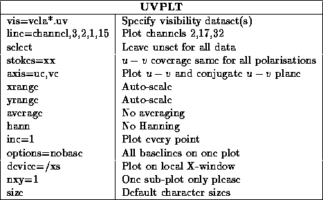
   The following example plots u versus v , and -u versus -v , selecting channels at the start, middle and end of a band of 32 channels (so that the u-v coverage benefit obtained across the band can be seen).

   

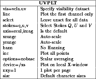
   The next example shows how to plot a scatter diagram (real vs imaginary) from a single-channel dataset for the Q , U and V . polarisations, with all baselines plotted on the one plot. This is a quite useful plot to make of calibrated calibrator data. Because you are asking for Stokes parameters, it is assumed that a calibration has been made (the calibration tables will be applied by uvplt and a reminder issued) or that you converted to Stokes parameters along the way (e.g. with the AIPS task ATLOD or with uvaver ).

   

2.  

   Task closure is another useful plotting task. It is most useful for plotting the closure phases of point sources. The closure phase of an object is the sum of the baseline phases around a triangle. For example, for antennas 1, 2 and 3 we measure three baseline phases , and . It can be shown that the closure phase, which is the sum of these three baseline phases

   

   will be independent of any antenna-based gain errors (atmosphere and instrumental). This quantity will not be affected by MIRIAD 's antenna calibration process. Additionally for a point source (or any source with 180 degree rotational symmetry) the closure phase should be zero. Plotting the closure phase of a calibrator is thus a way of checking the quality of the data. If the closure phase is large, the data are probably bad, or there is some calibration error that is not accounted for in MIRIAD 's antenna-based model.

   Task closure plots averages of closure phases (actually it averages together triple products and then takes the phase of this). The averages are taken over the the different correlator channels and polarisations, and optionally over time.

   The inputs to closure are simple enough. See the help file for more information. Typical inputs to uvtriple are:

   

3.   If you are working with spectral data (line or continuum) you may want to look at some spectra. Use task uvspec   for this. The inputs to uvspec are pretty much self-explanatory. Here is an example of how to plot the spectra (phase) of the XX and YY correlations averaged over 15 minutes for all baselines involving antenna 1 with all calibration turned off. uvspec makes a new sub-plot every time it begins a new averaging interval. Assuming that there are five antennas in this dataset, we have arranged for each baseline to occupy one column of the plot page with time increasing down the page.