Mosaicing Observing Strategies

• Pointing grid pattern: In a mosaic experiment, you observe a number of pointings -- possibly a few to several hundred, depending on the size of the source of interest. To consider how dense the sampling grid needs to be, consider the primary beam of an antenna. In the u-v plane, the Fourier transform of the primary beam pattern is just the cross-correlation between two antenna illumination patterns. For the 22-m ATCA dishes, the Fourier transform of the primary beam pattern will be of finite and circular extent, having a diameter of 44-m. Because it is of finite extent, Nyquist's sampling theorem indicates that, provided we do not sample in the sky domain coarser than some limit (i.e. provided the pointing grid pattern is sufficiently fine), all information can be retrieved. Assuming a standard, rectangular grid, the sky plane Nyquist sampling limit is

  

  ( is the wavelength, and D is the dish diameter). For a well-illuminated dish, this spacing corresponds roughly to half-power point spacing between field centres. Because the extent of the transform is circular, we can do somewhat better than this, by using a so-called hexagonal grid. This grid places pointing centres at the vertices of equilateral triangles -- packing six triangles together gives a hexagon. An extension of Nyquist's theorem indicates that

  

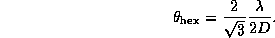
  So a hexagonal grid allows a given area of the sky to be covered in a smaller number of pointings (it does also require slightly longer drive times between pointings -- see below -- which may occassionally be a consideration). Table 20.1 gives this grid spacing for ATCA dishes.

    
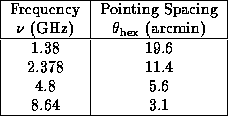
  Table 20.1: Mosaic grid spacing for ATCA dishes
  

• Dwell time: Most mosaiced experiments will continually switch between the different pointing centres (or a subset of them, if there are too many pointing centres to visit in a single observation). Normally they will be visited in a raster scan fashion. Switching to a new pointing centre typically results in 0.5 to 4 seconds of `lost' time while the antennas are slewing to the new pointing. This time can be a significant consideration in some experiments -- e.g. if the integration time was 10 seconds, and the pointing centre was switched every integration, up to about 40% of the observing time could be lost. To avoid this, you will want to dwell on a given pointing centre for as long as reasonable. This must, however, be traded against loss of tangential u-v coverage that occurs when each pointing is not visited sufficiently frequently. To determine the balance, recall that a correlation does not measure the value of a single point in the u-v plane, but a region corresponding to twice the diameter of the dishes. At transit (when the projected baselines are changing fastest), the time taken for a baseline to rotate to a completely independent visibility point is

  

  Here L is the maximum baseline length of interest when imaging and D is the dish diameter. Ideally you will want to sample twice as frequently as this, i.e. for N pointings, a dwell time of would be best. You may, however, decide to suffer tangential holes in the u-v coverage.

• Field Naming Convention: When preparing the observe files for an ATCA mosaic experiment, you will create a `mosaic file'. This gives a field offset, integration time and field name for each pointing centre. To simplify a step in the reduction process (the splitting step only), it is recommended that field names be composed of two parts, separated by an underscore character. This recommendation is purely to simplify some steps in the data reduction in MIRIAD . The first part should be common to all fields. Typically this will be the name of the object being mosaiced. The second part is unique to each field, typically being a field number. For example, the field name for pointing 123 for a Large Magellanic Cloud mosaic would be called lmc_123.