1. Introduction

As young objects are found in regions of enhanced gas density, it seems most likely that the SFR increases with the current local gas density. Schmidt (1959, 1963) finds a quadratic dependence on the mass density of H I gas: Ψ∝ρ². Madore et al. (1974) argue for a dependence on surface density, and Donas et al. (1987) derive a linear dependence of the total SFR of a galaxy and the mass of its atomic gas. But there is also evidence that the molecular gas is more responsible for the SFR (e.g. Guibert et al. (1978) and Rana & Wilkinson (1986) find exponents larger than 1 for the molecular mass density).

There may well be other quantities the SFR depends on: Talbot (1980) proposes that the SFR in the disk of a galaxy is proportional to the frequency with which the gas passes through spiral arms. Considerations of the stability of gas disks (cf. Kennicutt 1989) also give rise to an explicit dependence on radial distance. Wyse & Silk (1989) generalize this approach by also allowing a dependence on the gas surface density. Dopita (1985), Dopita & Ryder (1994), and Ryder & Dopita (1994) suggest a dependence on the total mass surface density.

Furthermore, there are both observational and theoretical indications for a minimum density or pressure for the SFR (cf. Kennicutt 1989; van der Hulst et al. 1993; Elmegreen & Parravano 1994; Kennicutt et al. 1994; Wang & Silk 1994; Chamcham & Hendry 1996). Above that threshold density, Kennicutt (1989) finds a SFR depending nearly linearly on total gas density (exponent of 1.3±0.3).

Theory has not been able to give firm predictions of the SFR much beyond providing possible identifications of plausible physical processes in order to explain the observed trends (cf. Franco 1990). A rather attractive concept is that the SFR is in fact the consequence of a self-regulation in a network of processes in the interstellar medium in the galactic environment. Several scenarios for such an equilibrium have been discussed (e.g. Cox 1983; Franco & Cox 1983; Franco & Shore 1984; Dopita 1985; Firmani & Tutukov 1992; Köppen et al. 1995, 1998), but a unique and precise prediction independent of observations is hard to get.

Which is the true law of star formation? Evidently, it is the one which gives the best fit to the data. But suppose one has 10 data points. While a simple prescription with a single fit parameter may already give an acceptable fit, it is surely improved by introducing another free parameter, and it could be made even better with a third one, ..... and so on. Finally we come up with a perfect fit using 10 free parameters - which is bound to encounter a general disbelief! How many parameters can be extracted from data? Statistical tests (like χ²-test) can only tell us when to reject too poor a fit, but there is nothing to indicate when a fit is too good. Usually, this decision is made more or less subjectively, based on one's feeling and experience: The metaphor of Occam's razor - of leaving out any complexity in a model unnecessary to explain the facts - is well known as a philosophical concept, but can one devise a practical, objective, and mathematically correct method to aid in this judgement?

Yes! It is the Bayesian approach to statistics that permits to formulate Occam's razor without introducing any artificial assumptions or subjective constructs, but in a natural and mathematically fully consistent way (Köppen & Fröhlich 1997). This method is applied to our principal question: Can we with the existing observational data decide between a SFR law which depends only on local gas surface density Ψ∝g^x with a fixed or free parameter x and a law which also has an explicit radial dependence Ψ∝g^x/r^y (y=1 corresponds to a flat rotation curve in the concept of Wyse & Silk)?

2. A Bayesian Method

The probabilities are computed with Bayes' Theorem (which is strictly valid in either view!): Let us consider a set of N hypotheses H_i, only one of which can be true. Then the probability for the k-th hypothesis, taking into account the data D, is

where 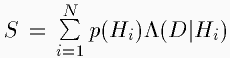is a normalizing factor. The prior probabilities p(H_k) represent the investigator's degree of belief or his knowledge from previous measurements. The likelihood Λ(D|H_k) is a measure of how well the predictions of H_k match the data, which incorporates the distribution functions of the random errors. Thus, Eq. (1) describes how a measurement improves our knowledge: It states that the posterior probability for a hypothesis is proportional to the product of its probability assigned before the observation and the likelihood Λ(D|H_k) of the data D.

In practice, one compares a few specific models, and so the set of hypotheses is not exhaustive. Therefore, only ratios of probabilities can be calculated, but as long as one sticks to the same set of models, explicit calculation of the normalizing sum S is unnecessary. It suffices to compute the numerator in Eq. (1), called the Bayes factor.

The correct formulation of the priors must include all previous knowledge. Since this is not easily derived from mathematical axioms, the classical approach prefers not to include the prior information at all, and is content by maximising the likelihood, and therefore is unable to compute the true posterior.

When a hypothesis contains free parameters λ, Bayes' Theorem gives the posterior density p(H_k, λ |D). This is integrated over the space of the parameters to get the probability for the hypothesis irrespective of the parameter's actual value:

where p(λ) is the prior probability density for the parameter. Since this prior is normalised over the parameter space 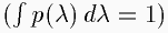the posterior decreases, if the parameter space is increased much beyond the volume where the likelihood density Λ(D|H_k,λ) contributes significantly. In this way, the increased freedom to get a good fit may well more than compensate any increase of the likelihood itself due to the better fit. It is this feature, naturally occurring in the Bayesian approach by taking seriously the prior information, which allows a mathematically consistent formulation of Occam's razor.

Equation (2) also shows that problems with many free parameters quickly lead to a heavy load of computer resources, because of the evaluation of multiple integrals. Wherever possible, analytical evaluation of some of the integrals thus is highly recommended.

Thinking about the formulation of the priors I found to be a most wholesome and enlightening exercise to make oneself aware of what one knows or not, or pretends to do so. For our question, we have used the following recipe. The parameter priors are taken from Jeffreys (1983) formulations for the absence of any prior information: Parameters which are simple numbers such exponents, a uniform prior density p(λ) = const. is taken. Dimensioned parameters (scalelengths, timescales, ..) follow a prior uniform in ln(λ), i.e. p(λ)∝1/λ.

The theory priors would be the place to formulate a possible (personal) preference of theories with a smaller number of free parameters. We take all hypotheses - irrespective of the number of their parameters - as equally preferable: p(H_k) = const.

For the treatment of nuisance parameters which are parameters of the problem or the model but whose values are of no interest to us - here: the factor between Halpha-brightness and SFR, and the size of the scatter in the data due to noise or intrinsic fluctuations of the SFR - and practical aspects of the integrations see Köppen & Fröhlich (1997, 1998).

3. Results on Halpha-density

Since our method yields proper probabilities (and densities), they can be used in a straightforward manner to calculate joint probabilities. Figure 2 shows the confidence region for the probability that the same pair (x,y) of parameters fits the data of all 12 galaxies. This region is quite small, with a peak corresponding to no radial dependence but a nearly linear dependence with gas density. The figure also shows that the choice of the CO-H₂ conversion does not greatly change this finding.

Likewise, probabilities for various sub-hypotheses can be obtained. In the Table we collect the joint Bayes factors for various laws with no, one, or two free parameters. This is done for the parameter either allowed to vary between individual galaxies or to have a value common for all objects. The ranges of the parameters are as shown in Fig. 1. All Bayes factors are normalized relative to the simple linear law

SFR-law	individual	common value
g	1
g2	1.9·10-6
g/r	1.3·10-15
gx	0.59	0.061
gx/r	2.0·10-13	4.1·10-12
g/ry	1.5·10-5	0.033
g2/ry	4.5·10-7	0.002
gx/ry	9.8·10-6	0.002
xbest	-	0.73
ybest	-	-0.06

One notes that the most likely laws are the simple linear law and the dependence on gas density where each galaxy has its own optimal exponent. Laws like g² or g/r are in quite strong disagreement with the observational data, and so are the other laws.

If one reduced the assumed parameter range for x of (-6 ... 11) by say a factor 2, the Bayes factors of laws with common parameter values for all galaxies would be approximately doubled - the parameter prior is applied only once. On the other hand, for the laws whose parameters are allowed to vary individually among the 12 galaxies the prior is applied for each object, so the factors would increase by about 2¹²≅4000. In this manner, these laws could be made more probable. But this merely reflects their much larger freedom for making the fit as compared to laws where the same parameter value is to be used for all objects.

4. The Gas Fraction

First, a direct analysis of the data from each galaxy is done, as shown in Fig. 3 for the Milky Way as a typical example: Most of the galactic disk (from 3 to 12 kpc) has not only a nearly constant gas fraction of about 7 percent, but also a nearly constant ratio of Halpha-brightness and (total) gas density - i.e. the current SFR is simply proportional to the gas density. Outside this region of the disk, the SFR is much lower, and the gas fraction quite different: e.g. inside 3 kpc (filled circle) there is little gas. With a few exceptions, the other galaxies show quite similar behaviour. This suggests that in the ring of the disk where most of `normal' star formation occurs, the SFR is rather close to a simple linear dependence of the gas density.

In nearly all galaxies the gas fraction increases only very gently towards the exterior, as shown in Fig. 4.

That the linear SFR has been responsible for all previous star formation in the disk, is the simplest explanation for this shallow variation of the gas fraction: Assuming a closed-box model with initial gas density g₀(r) for each radial ring, one gets with a general SFR Ψ = C(r)·g^x for an age t:

A nearly constant f_gas = g/g₀ requires

If all sections of the disk have the same age t, the linear dependence of the SFR on gas density (x=1 and C(r)=const.) provides an easy explanation.

The Bayesian method is applied to the comparison of the observed radial profiles of stellar and gas density with models where the disk is formed by gas infall and where gas is allowed to flow outward in radial direction, and star formation follows the two-parameter law as before. Figure 5 shows the contour lines in the space of parameters (x,y) of the probability density integrated over all remaining (four) parameters. These first results show that the 90 percent confidence regions are much smaller that those obtained from the Halpha-data, and they keep very close to the simple linear law (x≅1...2 and y≅0). This finding appears to be not very sensitive to other model parameters, such as infall and gas flows, though the probability obtained does vary, of course.

5. Conclusions

With respect to irregular and dwarf galaxies, one may envisage to unravel the history of the starburst activity or to find out which spatial and temporal relations between star forming regions may be deducible. The method outlined here can be applied for any comparison of models with data, providing from the observations themselves a good indication of whether a certain model is justified or might come close to an over-interpretation.

References

• Arimoto N., Sofue Y., Tsujimoto T., 1996, PASJ 48, 275
• Chamcham K., Hendry M.A., 1996, MNRAS 279, 1083
• Cox D.P., 1983, ApJ 265, L61
• Dopita M.A., 1985, ApJ 295, L5
• Dopita M.A., Ryder S.D., 1994, ApJ 430, 163
• Donas J., Deharveng J.M., Laget M., Milliard B., Huguenin D., 1987, A&A 180, 12
• Elmegreen B.G., Parravano A., 1994, ApJ 435, L121
• Erickson G.J., Smith C.R. (eds.), 1988, Maximum-Entropy and Bayesian Methods in Science and Engineering, Kluwer, Dordrecht
• Firmani C., Tutukov A., 1992, A&A 264, 37
• Franco J., 1990, in 'Chemical and Dynamical Evolution of Galaxies', Ferrini F., Franco J., Matteucci F. (eds.), ETS editrice, Pisa
• Franco J., Cox D.P., 1983, ApJ 273, 243
• Franco J., Shore S.N., 1984, ApJ 285, 213
• Fougère P.F. (ed.), 1990, Maximum Entropy and Bayesian Methods, Kluwer, Dordrecht
• Guibert J., Lequeux J., Viallefond F., A&A 68, 1
• Jeffreys H., 1983, Theory of Probability, 3rd ed., Clarendon Press, Oxford
• Kennicutt R.C., 1989, ApJ 344, 685
• Kennicutt R.C., Tamblyn P., Congdon C.W., 1994, ApJ 435, 22
• Köppen J., Fröhlich H.-E., 1997, A&A 325, 961
• Köppen J., Theis Ch., Hensler G., 1995, A&A 296, 99
• Köppen J., Theis Ch., Hensler G., 1998, A&A 331, 524
• Madore B.F., van den Bergh S., Rogstad D., 1974, ApJ 191, 317
• O'Hagan A., 1994, Kendall's Advanced Theory of Statistics, Vol. 2B, Bayesian Inference, Edward Arnold, London
• Rana N.C., Wilkinson D.A., 1986, MNRAS 218, 497
• Ryder S.D., Dopita M.A., 1994, ApJ 430, 142
• Schmidt M., 1959, ApJ 129, 243
• Schmidt M., 1963, ApJ 137, 758
• Talbot R.J., 1980, ApJ 235, 821
• van der Hulst J.M., Skillman E.D., Smith T.R., et al., 1993, AJ 106, 548
• Wang B., Silk J., 1994, ApJ 427, 759
• Wyse R.F.G., Silk J., 1989, ApJ 339, 700

• Content of the GK Workshop Proceedings
• Programme of the GK Workshop
• List of Participants
• Graduiertenkolleg - home page
• Astronomische Institute der Universität Bonn (AIUB)