Much of the theory here has been borrowed from the memo `AT Polarisation Calibration' (Bob Sault, Neil Killeen and Mike Kesteven). See that memo for more details. A more detailed description of polarimetric interferometry can be found in Hamaker, Bregman & Sault and Sault, Hamaker & Bregman (A&ASS 1996).
Recall from Chapter 5 that MIRIAD models a feed as having a composite gain of

where g(t)
is a time variable complex number (often loosely called the
antenna gain),  is the bandpass function, and
  is a
time-varying delay term.
is a
time-varying delay term.
Additionally, we have to consider the response of the feeds to polarised emission. Whether a feed is linearly or circularly polarised, its instantaneous response to a signal is a linear combination of two of the four Stokes parameters that describe the wave. In the equatorial frame of the source, ideal linear feeds respond according to
where the X and Y feeds are at position angles 0 and 90, respectively. Perfect circular feeds respond according to
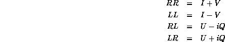
These equations show immediately why it is harder to calibrate an instrument with linear feeds, such as the ATCA, compared with an instrument with circular feeds, such as the VLA. In the latter case, one can make the excellent assumption that the calibrators, which are used to determine the antenna gains, are not circularly polarised. Thus, the RR and LL visibilities are a direct measure of I , for which we have a good model ( i.e. a point source of known flux density). Consequently they can be used to calibrate the gains with time. On the other hand, it is not necessarily a good assumption that a calibrator is not linearly polarised, so that XX and YY correlations cannot always be used as a direct measure of I .
In addition, for `alt-az' telescopes, the feeds rotate with respect to the
equatorial frame. This causes the actual response of ideal linearly
polarised feeds to vary with the parallactic angle,  (which
varies with time, although non-linearly), according to
(which
varies with time, although non-linearly), according to
So far we have assumed that the feeds are ideal. This is never the
case, and their departure from the ideal can be characterized by
leakage terms.  is the leakage of the y
component of the
electric field into the X
feed, and
is the leakage of the y
component of the
electric field into the X
feed, and  is the leakage of the x
component of the electric field into the Y feed. Another way of thinking of them is the combination of the ellipticity and error in the position angle of the polarisation ellipses of each feed.
Incorporating these terms, neglecting all terms involving the product of leakage terms, and showing the gains ( g ) explicitly, one can show that the linear correlations are
where the subscripts i
and j
denote the two antennas involved in the
visibility. The left-hand sides of these equations, the leakage ( D
)
terms, and gains ( g
) are all complex. I
, Q
, U
, and V
are real
numbers. Note how the leakage terms corrupt the correlations in two
ways. First, there are sinusoids with parallactic angle with amplitudes
given by Q
and U
. Second, there are constant terms which are
fractions of I
and V
. The XY
phases
are the difference between the phases of the  and
and  gains;
this is an antenna-based quantity.
gains;
this is an antenna-based quantity.
Inverting these equations gives an even longer set of equations that describe the Stokes parameters, each a linear combination of the four correlations. Here they are for reference, ignoring the gain terms