Computation

Task invert is a fairly conventional imaging program, which produces a dirty image from a visibility dataset. It normally does this using a grid-and-FFT approach, although there are switches to use a direct Fourier transform and a median algorithm. Task invert

does not require the data to be sorted in any way. Normally any calibration tables are applied by invert on-the-fly (although this can be turned off with the nocal, nopol and nopass options). Both continuum or spectral line observations are handled.

We describe the inputs to invert . For MFS imaging, note options=mfs (and options=sdb) options.

• vis gives the name of the input visibility datasets. Several datasets can be given, as may be convenient when a source is observed with multiple configurations or multiple frequencies. The selected data are assumed to be of the same object, with the same pointing centre. Additionally, when making spectral line cubes, the number of channels derived from each dataset must be the same (this restriction does not apply for MFS images). Dataset names can include wildcards.

• map is the name of the output image dataset(s). When several Stokes parameters are being imaged, you need to give one name for each Stokes type. There is no default.

• beam is the name of the output beam dataset. The default is not to create an output beam. If you wish to deconvolve, then you must create an output beam. Note that invert produces a single beam which corresponds to all image planes and Stokes parameters.

• cell gives the image pixel size in arcseconds. Either one or two values can be given. If only one value is given, the pixels are square. The default is to choose a pixel size which samples the synthesised beam by about a factor of 3 (i.e. the recommended sampling for deconvolution).

• imsize gives the size of the images in pixels. It need not be a power of two. Generally the beam is also this size, but see options=double below.

• line is the normal data linetype selection. The default linetype is the first channel when performing normal imaging and all channels when doing multi-frequency synthesis. Generally you should set this parameter if you have more than one channel.

• select is the normal visibility data selection. The default is to select all data.

• stokes gives the Stokes or polarisation types to be imaged. Several values can be given, separated by commas. For example

       stokes=i,q,u,v
  

  will cause images of Stokes I , Q , U and V to be formed. Note that there needs to be a corresponding output file (see map above) for each Stokes parameter being imaged. The default Stokes parameter to image is `ii', which images Stokes-I, and assumes that the source is otherwise unpolarised.

• offset: This gives an offset, in arcseconds on the sky, to shift the image centre away from phase centre. Positive values result in the image centre being to the north and east of the observing centre. If one value is given, both RA and DEC are shifted by this amount. If two values are given, then they are the RA and DEC shifts. The default is no shift.

• options gives extra processing options. Several options can be given (abbreviated to uniqueness), separated by commas. Possible values are:

  mfs:

  This invokes multi-frequency synthesis imaging, as described above. All selected channels and frequencies will be gridded simultaneously to form a single output image.

  sdb:

  This is used in MFS imaging to cause invert to produce a spectral dirty beam (this is stored as a second plane of the beam data-set). The spectral dirty beam is used by the deconvolution task mfclean in determining the spectral index of the image. Generally if you think you may use mfclean to deconvolve your image, then you should set options=sdb. See the discussion of multi-frequency synthesis in Section 13.3 for more information.

  double:

  Normally invert makes a beam which is the same size as the image. However MIRIAD 's deconvolution tasks generally require a beam which is four times the area than the region being deconvolved. The double option causes invert to produce a beam which is twice the linear extent (four times the area) of the image. In this way, you can request invert to map just the region containing real emission, plus a guard band (at least 5 pixels on each edge).

  systemp:

  See the description in the weighting section above.

  nocal:

  By default, invert applies any gain calibration to the data before imaging. The nocal option turns off this step.

  nopass:

  By default, invert applies any bandpass calibration to the data before imaging. The nopass option turns off this step.

  nopol:

  By default, invert applies any polarisation leakage correction to the data before imaging. The nopol option turns off this step.

  mosaic:

  This invokes invert 's mosaic mode. See Chapter 20 for more information.

  imaginary:

  This makes the `imaginary' image. This is useful for non-Hermitian data (holography) or for investigating certain instrumental errors.

  amplitude:

  Set the phase of each visibility to zero before imaging.

  phase:

  Set the amplitude of each visibility to unity before imaging.

• mode: This determines the imaging algorithm to be used. Possible values are fft (a conventional grid and FFT imaging algorithm), dft (a direct Fourier transform approach) and median (a median Fourier transform). The dft approach produces fewer artifacts in the resultant images, but at substantial computational expense. The median approach os more robust to bad data and sidelobes, but at an even more substantial computational cost. The default mode is fft -- this should be used on all but the smallest datasets and images.

• slop: The slop factor. This is used in specrtal-line imaging. See Section 15.9 for more information.

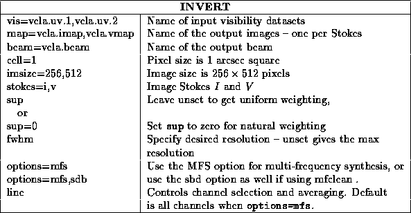
Typical inputs to invert for a continuum experiment are given below.

For a spectral line observation, typical inputs would be

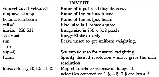
invert prints out a few numbers that may be of use -- the average system temperature, average system gain and theoretical rms noise. The theoretical rms noise is calculated assuming that the only source of error is the system temperature of the front-end receiver. No account is made of calibration errors, sidelobes or any other `instrumental' effects. The calculation correctly accounts for the weighting scheme used in the imaging process. This theoretical noise is the level you can expect in a detection experiment (assuming no interference or confusion), and it is the best one can hope for in high dynamic range work (usually instrumental effects will limit you before the noise in these sorts of experiments).

The noise calculation of invert (and all other MIRIAD tasks that compute the variance of a correlation) is based on values of system temperature, system gain, integration time and bandwidth stored in a dataset. Unfortunately data loaded into MIRIAD using fits will have only nominal system temperatures and system gains, and an educated guess is made for the integration time. Data loaded using MIRIAD atlod , the system temperatures are those measured on-line, and the integration time will be correct. See Chapter 8 for a discussion of setting you dataset up so that noise estimates are correct. The system gain, however, is still a nominal figure. If system temperature, system gain or integration time are incorrect by some factor, then the theoretical rms noise will also be wrong by a factor.

There is another effect which will cause invert 's noise estimate to be a factor of too pessimistic (i.e. the actual noise is a factor of lower than the printed value). With the ATCA correlator in its continuum (33 channel) mode, the channel bandwidth is twice as large as the separation between channels ( i.e. the channels are oversampled). Unfortunately invert assumes that the bandwidth is the same as the separation. This will only affect you if you are imaging individual correlator channels (i.e. no frequency averaging). It will not affect ``channel 0'' or multi-frequency synthesis imaging.